Higher Gauge Theory in Edinburgh – Part I

The main thing happening in my end of the world is that it’s relocated from Europe back to North America. I’m taking up a teaching postdoc position in the Mathematics and Computer Science department at Mount Allison University starting this month. However, amidst all the preparations and moving, I was also recently in Edinburgh, Scotland for a workshop on Higher Gauge Theory and Higher Quantization, where I gave a talk called 2-Group Symmetries on Moduli Spaces in Higher Gauge Theory. That’s what I’d like to write about this time.

Edinburgh is a beautiful city, though since the workshop was held at Heriot-Watt University, whose campus is outside the city itself, I only got to see it on the Saturday after the workshop ended. However, John Huerta and I spent a while walking around, and as it turned out, climbing a lot: first the Scott Monument, from which I took this photo down Princes Street:

And then up a rather large hill called Arthur’s Seat, in Holyrood Park next to the Scottish Parliament.

The workshop itself had an interesting mix of participants. Urs Schreiber gave the most mathematically sophisticated talk, and mine was also quite category-theory-minded. But there were also some fairly physics-minded talks that are interesting to me as well because they show the source of these ideas. In this first post, I’ll begin with my own, and continue with David Roberts’ talk on constructing an explicit string bundle. …

2-Group Symmetries of Moduli Spaces

My own talk, based on work with Roger Picken, boils down to a couple of observations about the notion of symmetry, and applies them to a discrete model in higher gauge theory. It’s the kind of model you might use if you wanted to do lattice gauge theory for a BF theory, or some other higher gauge theory. But the discretization is just a convenience to avoid having to deal with infinite dimensional spaces and other issues that don’t really bear on the central point.

Part of that point was described in a previous post: it has to do with finding a higher analog for the relationship between two views of symmetry: one is “global” (I found the physics-inclined part of the audience preferred “rigid”), to do with a group action on the entire space; the other is “local”, having to do with treating the points of the space as objects of a groupoid who show how points are related to each other. (Think of trying to describe the orbit structure of just the part of a group action that relates points in a little neighborhood on a manifold, say.)

In particular, we’re interested in the symmetries of the moduli space of connections (or, depending on the context, flat connections) on a space, so the symmetries are gauge transformations. Now, here already some of the physically-inclined audience objected that these symmetries should just be eliminated by taking the quotient space of the group action. This is based on the slogan that “only gauge-invariant quantities matter”. But this slogan has some caveats: in only applies to closed manifolds, for one. When there are boundaries, it isn’t true, and to describe the boundary we need something which acts as a representation of the symmetries. Urs Schreiber pointed out a well-known example: the Chern-Simons action, a functional on a certain space of connections, is not gauge-invariant. Indeed, the boundary terms that show up due to this not-invariance explain why there is a Wess-Zumino-Witt theory associated with the boundaries when the bulk is described by Chern-Simons.

Now, I’ve described a lot of the idea of this talk in the previous post linked above, but what’s new has to do with how this applies to moduli spaces that appear in higher gauge theory based on a 2-group . The points in these space are connections on a manifold . In particular, since a 2-group is a group object in categories, the transformation groupoid (which captures global symmetries of the moduli space) will be a double category. It turns out there is another way of seeing this double category by local descriptions of the gauge transformations.

In particular, general gauge transformations in HGT are combinations of two special types, described geometrically by -valued functions, or -valued 1-forms, where is the group of objects of , and is the group of morphisms based at . If we think of connections as functors from the fundamental 2-groupoid into , these correspond to pseudonatural transformations between these functors. The main point is that there are also two special types of these, called “strict”, and “costrict”. The strict ones are just natural transformations, where the naturality square commutes strictly. The costrict ones, also called ICONs (for “identity component oplax natural transformations” – see the paper by Steve Lack linked from the nlab page above for an explanation of “costrictness”). They assign the identity morphism to each object, but the naturality square commutes only up to a specified 2-cell. Any pseudonatural transformation factors into a strict and costrict part.

The point is that taking these two types of transformation to be the horizontal and vertical morphisms of a double category, we get something that very naturally arises by the action of a big 2-group of symmetries on a category. We also find something which doesn’t happen in ordinary gauge theory: that only the strict gauge transformations arise from this global symmetry. The costrict ones must already be the morphisms in the category being acted on. This category plays the role of the moduli space in the normal 1-group situation. So moving to 2-groups reveals that in general we should distinguish between global/rigid symmetries of the moduli space, which are strict gauge transformations, and costrict ones, which do not arise from the global 2-group action and should be thought of as intrinsic to the moduli space.

String Bundles

David Roberts gave a rather interesting talk called “Constructing Explicit String Bundles”. There are some notes for this talk here. The point is simply to give an explicit construction of a particular 2-group bundle. There is a lot of general abstract theory about 2-bundles around, and a fair amount of work that manipulates physically-motivated descriptions of things that can presumably be modelled with 2-bundles. There has been less work on giving a mathematically rigorous description of specific, concrete 2-bundles.

This one is of interest because it’s based on the String 2-group. Details are behind that link, but roughly the classifying space of (a homotopy 2-type) is fibred over the classifying space for (a 1-type). The exact map is determined by taking a pullback along a certain characteristic class (which is a map out of ). Saying “the” string 2-group is a bit of a misnomer, by the way, since such a 2-group exists for every simply connected compact Lie group . The group that’s involved here is a , the string 2-group associated to , the universal cover of the rotation group . This is the one that determines whether a given manifold can support a “string structure”. A string structure on , therefore, is a lift of a spin structure, which determines whether one can have a spin bundle over , hence consistently talk about a spin connection which gives parallel transport for spinor fields on . The string structure determines if one can consistently talk about a string-bundle over , and hence a 2-group connection giving parallel transport for strings.

In this particular example, the idea was to find, explicitly, a string bundle over Minkowski space – or its conformal compactification. In point of fact, this particular one is for $latek String(5)$, and is over 6-dimensional Minkowski space, whose compactification is . This particular is convenient because it’s possible to show abstractly that it has exactly one nontrivial class of string bundles, so exhibiting one gives a complete classification. The details of the construction are in the notes linked above. The technical details rely on the fact that we can coordinatize nicely using the projective quaternionic plane, but conceptually it relies on the fact that , and because of how the lifting works, this is also . This quotient means there’s a string bundle whose fibre is .

While this is only one string bundle, and not a particularly general situation, it’s nice to see that there’s a nice elegant presentation which gives such a bundle explicitly (by constructing cocycles valued in the crossed module associated to the string 2-group, which give its transition functions).

(Here endeth Part I of this discussion of the workshop in Edinburgh. Part II will talk about Urs Schreiber’s very nice introduction to Higher Geometric Quantization)

(This ends the first part of this update – the next will describe the physics-oriented talks, and the third will describe Urs Schreiber’s series on higher geometric quantization)

 

TQFT’s in Vienna – Part 1

So I spent a few weeks at the Erwin Schrodinger Institute in Vienna, doing a short residence as part of the program “Modern Trends in Topological Quantum Field Theory” leading up to a workshop this week. There were quite a few interesting talks – some on topics that I’ve written about elsewhere in this blog, so I’ll gloss over those. For example, Catherine Meusburger spoke about the project with Barrett and Schaumann to give a diagrammatic language for Gray categories with duals – I’ve written about John Barrett’s talks on this elsewhere. Similarly, I’ve written about Chris Schommer-Pries’ talks about fully-extended TQFT’s and the cobordism hypothesis for structured cobordisms . I’d like to just describe some of the other highlights that connect nicely to themes I find interesting. In Part 1 of this post, the more topological themes…

TQFTs with Boundary

On the first day, Kevin Walker gave a talk called “Premodular TQFTs” which was quite interesting. The key idea here is that a fairly big class of different constructions of 3D TQFT’s turn out to actually be aspects of one 4D TQFT, which comes about by a construction based on the 3D construction of Crane-Yetter-Kauffman.  The term “premodular” refers to the fact that 3D TQFT’s can be related to modular tensor categories. “Tensor” includes several concepts, like being abelian, having vector spaces of morphisms, a monoidal structure that gets along with these – typical examples being the categories of vector spaces, or of representations of some fixed group. “Modular” means that there is a braiding, and that a certain string diagram (which looks like two linked rings) built using the braiding can be represented as an invertible matrix. These will show up as a special case of the “premodular” theory.

The basic idea is to use an approach that is based on local fields (which respects the physics-land concept of what “field theory” means), avoids the path integral approach (which is hard to make rigorous), and can be shown to connect back to the Atyiah-Singer approach in which a TQFT is a kind of functor out of a cobordism category.

That is, given a manifold we must be able to find the fields on , called . For example, could be the maps into a classifying space , for a gauge theory, or a category of diagrams on with labels in some appropriate sort of category. Then one has some relations which say when given fields are the same. For each manifold , this defines a vector space of linear combinations of fields, modulo relations, called , where . The dual space of is called – in keeping with the principle that quantum states are functionals that we can evaluate on “classical” fields.

Walker’s talk develops, from this starting point, a view that includes a whole range of theories – the Dijkgraaf-Witten model (fields are maps to ); diagrams in a semisimple 1-category (“Euler characteristic theory”), in a pivotal 2-category (a Turaev-Viro model), or a premodular 3-category (a “Crane-Yetter model”), among others. In particular, some familiar theories appear as living on 3D boundaries to a 4D manifold, where such a  premodular theory is defined. The talk goes on to describe a kind of “theory with defects”, where two different theories live on different parts of a manifold (this is a common theme to a number of the talks), and in particular it describes a bimodule which gives a Morita equivalence between two sorts of theory – one based on graphs labelled in representations of a group , and the other based on -connections. The bimodule is, effectively, a kind of “Fourier transform” which relates dimension- structures on one side to codimension- structures on the other: a line labelled by a -representation on one side gets acted upon by -holonomies for a hypersurface on the other side.

On a related note Alessandro Valentino gave a talk called “Boundary Conditions for 3d TQFT and module categories” This related to a couple of papers with Jurgen Fuchs and Christoph Schweigert. The basic idea starts with the fact that one can build (3,2,1)-dimensional TQFT’s from modular tensor categories , getting a Reshitikhin-Turaev type theory which assigns to the circle. The modular tensor structure tells you what gets assigned to higher-dimensional cobordisms. (This is a higher-categorical analog of the fact that a (2,1)-dimensional TQFT is determined by a Frobenius algebra). Then the motivating question is: how can we extend this theory all the way down to a point (i.e. have it assign something to a point, so that is somehow composed of naturally occurring morphisms).

So the question is: if we know what is, what does that tell us about the “colours” that could be assigned to a boundary. There’s a fairly elegant way to take on this question by looking at what’s assigned to Wilson lines, the observables that matter in defining RT-type theories, when the line where we’re observing gets pushed onto the boundary. (See around p14 of the first paper linked above). The colours on lines inside the manifold could be objects of , and fusing them illustrates the monoidal structure of . Then the question is what kind of category can be attached to a boundary and be consistent with this.This should be functorial with respect to fusing two lines (i.e. doing this before or after projecting to the boundary should be the same).

They don’t completely characterize the situation, but they give some reasonable arguments which suggest that the result is that the boundary category, a braided monoidal category, ought to be the Drinfel’d centre of something. This is actually a stronger constraint for categories than groups (any commutative group is the centre of something – namely itself – but this isn’t true for monoidal categories).

2-Knots

Joost Slingerland gave a talk called “Local Representations of the Loop Braid Group”, which was quite nice. The Loop Braid Group was introduced by the late Xiao-Song Lin (whom I had the pleasure to know at UCR) as an interesting generalization of the braid group . is the “motion group” of isomorphism classes of motions of particles in a plane: in such a motion, we let the particles move around arbitrarily, before ending up occupying the same points occupied initially. (In the “pure braid group”, each individual point must end up where it started – in the braid group, they can swap places). Up to diffeomorphism, this keeps track of how they move around each other – not just how they exchange places, but which one crosses in front of which, etc. The loop braid group does the same for loops embedded in 3D space. Now, if the loops always stay far away from each other, one possibility is that a motion amounts to a permutation in which the loops switch places: two paths through 3D space (or 4D spacetime) can always be untangled. On the other hand, loops can pass THROUGH each other, as seen at the beginning of this video:

This is analogous to two points braiding in 2D space (i.e. strands twisting around each other in 3D spacetime), although in fact these “slide moves” form a group which is different from just the pure braid group – but fits inside them. In particular, the slide moves satisfy some of the same relations as the braid group – the Yang-Baxter equations.

The final thing that can happen is that loops might move, “flip over”, and return to their original position with reversed orientation. So the loop braid group can be broken down as . Every loop braid could be “closed up” to a 4D knotted surface, though not every knotted surface would be of this form. For one thing, our loops have a trivial embedding in 3D space here – to get every possible knotted surface, we’d need to have knots and links sliding around, braiding through each other, merging and splitting, etc. Knotted surfaces are much more complex than knotted circles, just as the topology of embedded circles is more complex than that of embedded points.

The talk described some work on the “local representations” of : representations on spaces where each loop is attached some -dimensional vector space (this is the “local dimension”), so that the motions of loops gets represented on (a tensor product of copies of ). This is already rather complex, but is much easier than looking for arbitrary representations of on any old vector space (“nonlocal” representations, if you like). Now, in particular, for local dimension 2, this boils down to some simple matrices which can be worked out – the slide moves are either represented by some permutation matrices, or some tensor products of rotation matrices, or a few other cases which can all be classified.

Toward the end, Dror Bar-Natan also gave a talk that touched on knotted surfaces, called “A Partial Reduction of BF Theory to Combinatorics“. The mention of BF theory – a kind of higher gauge theory that can be described locally in terms of a 1-form and a 2-form on a manifold – is basically to set up some discussion of knotted surfaces (the combinatorics it reduces to). The point is that, like many field theories, BF theory amplitudes can be calculated using a sum over certain Feynman diagrams – but these ones are diagrams that lie partly in certain knotted surfaces. (See the rather remarkable handout in the link above for lots of pictures). This is sort of analogous to how some gauge theories in 3D boil down to knot invariants – for knots that live on the boundary of a region cut out of the 3-manifold. This is similar, for a knotted surface in a 4-manifold.

The “combinatorics” boils down to showing some diagram presentations of these knotted surfaces – particularly, a special type called a “ribbon knot”, which is a certain kind of knotted sphere. The combinatorics show that these special knotted surfaces all correspond to ordinary knotted circles in 3D (in the handout, you’ll see the Gauss diagram for a knot – a picture which shows which points along a line cross over or under each other in a presentation of the knot – used to construct a corresponding ribbon knot). But do check out the handout for some pictures which show several different ways of presenting 2-knots.

(…To be continued in Part 2…)

 

Categorifying Global vs. Local Symmetry

So it’s been a while since I last posted – the end of 2013 ended up being busy with a couple of visits to Jamie Vicary in Oxford, and Roger Picken in Lisbon. In the aftermath of the two trips, I did manage to get a major revision of this paper submitted to a journal, and put this one out in public. A couple of others will be coming down the pipeline this year as well.

I’m hoping to get back to a post about motives which I planned earlier, but for the moment, I’d like to write a little about the second paper, with Roger Picken.

Global and Local Symmetry

The upshot is that it’s about categorifying the concept of symmetry. More specifically, it’s about finding the analog in the world of categories for the interplay between global and local symmetry which occurs in the world of set-based structures (sets, topological spaces, vector spaces, etc.) This distinction is discussed in a nice way by Alan Weinstein in this article from the Notices of the AMS from

The global symmetry of an object in some category can be described in terms of its group of automorphisms: all the ways the object can be transformed which leave it “the same”. This fits our understanding of “symmetry” when the morphisms can really be interpreted as transformations of some sort. So let’s suppose the object is a set with some structure, and the morphisms are set-maps that preserve the structure: for example, the objects could be sets of vertices and edges of a graph, so that morphisms are maps of the underlying data that preserve incidence relations. So a symmetry of an object is a way of transforming it into itself – and an invertible one at that – and these automorphisms naturally form a group . More generally, we can talk about an action of a group on an object , which is a map .

“Local symmetry” is different, and it makes most sense in a context where the object is a set – or at least, where it makes sense to talk about elements of , so that has an underlying set of some sort.

Actually, being a set-with-structure, in a lingo I associate with Jim Dolan, means that the forgetful functor is faithful: you can tell morphisms in (in particular, automorphisms of ) apart by looking at what they do to the underlying set. The intuition is that the morphisms of are exactly set maps which preserve the structure which forgets about – or, conversely, that the structure on objects of is exactly that which is forgotten by . Certainly, knowing only this information determines up to equivalence. In any case, suppose we have an object like this: then knowing about the symmetries of amounts to knowing about a certain group action, namely the action of , on the underlying set .

From this point of view, symmetry is about group actions on sets. The way we represent local symmetry (following Weinstein’s discussion, above) is to encode it as a groupoid – a category whose morphisms are all invertible. There is a level-slip happening here, since is now no longer seen as an object inside a category: it is the collection of all the objects of a groupoid. What makes this a representation of “local” symmetry is that each morphism now represents, not just a transformation of the whole object , but a relationship under some specific symmetry between one element of and another. If there is an isomorphism between and , then and are “symmetric” points under some transformation. As Weinstein’s article illustrates nicely, though, there is no assumption that the given transformation actually extends to the entire object : it may be that only part of has, for example, a reflection symmetry, but the symmetry doesn’t extend globally.

Transformation Groupoid

The “interplay” I alluded to above, between the global and local pictures of symmetry, is to build a “transformation groupoid” (or “action groupoid“) associated to a group acting on a set . The result is called for short. Its morphisms consist of pairs such that  is a morphism taking to its image under the action of . The “local” symmetry view of treats each of these symmetry relations between points as a distinct bit of data, but coming from a global symmetry – that is, a group action – means that the set of morphisms comes from the product .

Indeed, the “target” map in from morphisms to objects is exactly a map . It is not hard to show that this map is an action in another standard sense. Namely, if we have a real action , then this map is just , which moves one of the arguments to the left side. If was a functor, then $\hat{\phi}$ satisfies the “action” condition, namely that the following square commutes:

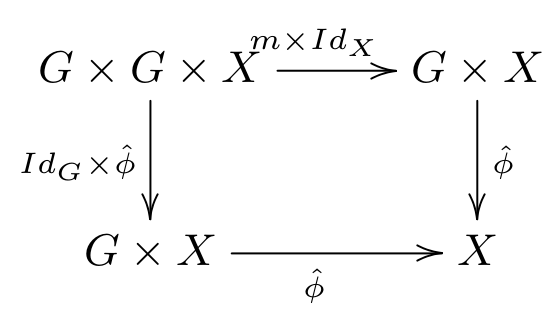
(Here, is the multiplication in , and this is the familiar associativity-type axiom for a group action: acting by a product of two elements in is the same as acting by each one successively.

So the starting point for the paper with Roger Picken was to categorify this. It’s useful, before doing that, to stop and think for a moment about what makes this possible.

First, as stated, this assumed that either is a set, or has an underlying set by way of some faithful forgetful functor: that is, every morphism in corresponds to a unique set map from the elements of to itself. We needed this to describe the groupoid , whose objects are exactly the elements of . The diagram above suggests a different way to think about this. The action diagram lives in the category : we are thinking of as a set together with some structure maps. and the morphism must be in the same category, , for this characterization to make sense.

So in fact, what matters is that the category lived in was closed: that is, it is enriched in itself, so that for any objects , there is an object , the internal hom. In this case, it’s which appears in the diagram. Such an internal hom is supposed to be a dual to ‘s monoidal product (which happens to be the Cartesian product ): this is exactly what lets us talk about .

So really, this construction of a transformation groupoid will work for any closed monoidal category , producing a groupoid in . It may be easier to understand in cases like , the category of topological spaces, where there is indeed a faithful underlying set functor. But although talking explicitly about elements of was useful for intuitively seeing how relates global and local symmetries, it played no particular role in the construction.

Categorify Everything

In the circles I run in, a popular hobby is to “categorify everything“: there are different versions, but what we mean here is to turn ideas expressed in the world of sets into ideas in the world of categories. (Technical aside: all the categories here are assumed to be small). In principle, this is harder than just reproducing all of the above in any old closed monoidal category: the “world” of categories is , which is a closed monoidal 2-category, which is a more complicated notion. This means that doing all the above “strictly” is a special case: all the equalities (like the commutativity of the action square) might in principle be replaced by (natural) isomorphisms, and a good categorification involves picking these to have good properties.

(In our paper, we left this to an appendix, because the strict special case is already interesting, and in any case there are “strictification” results, such as the fact that weak 2-groups are all equivalent to strict 2-groups, which mean that the weak case isn’t as much more general as it looks. For higher -categories, this will fail – which is why we include the appendix to suggest how the pattern might continue).

Why is this interesting to us? Bumping up the “categorical level” appeals for different reasons, but the ones matter most to me have to do with taking low-dimensional (or -codimensional) structures, and finding analogous ones at higher (co)dimension. In our case, the starting point had to do with looking at the symmetries of “higher gauge theories” – which can be used to describe the transport of higher-dimensional surfaces in a background geometry, the way gauge theories can describe the transport of point particles. But I won’t ask you to understand that example right now, as long as you can accept that “what are the global/local symmetries of a category like?” is a possibly interesting question.

So let’s categorify the discussion about symmetry above… To begin with, we can just take our (closed monoidal) category to be , and follow the same construction above. So our first ingredient is a 2-group . As with groups, we can think of a 2-group either as a 2-category with just one object , or as a 1-category with some structure – a group object in , which we’ll call if it comes from a given 2-group. (In our paper, we keep these distinct by using the term “categorical group” for the second. The group axioms amount to saying that we have a monoidal category . Its objects are the morphisms of the 2-group, and the composition becomes the monoidal product .)

(In fact, we often use a third equivalent definition, that of crossed modules of groups, but to avoid getting into that machinery here, I’ll be changing our notation a little.)

2-Group Actions

So, again, there are two ways to talk about an action of a 2-group on some category . One is to define an action as a 2-functor . The object being acted on, , is the unique object – so that the 2-functor amounts to a monoidal functor from the categorical group into . Notice that here we’re taking advantage of the fact that is closed, so that the hom-“sets” are actually categories, and the automorphisms of – invertible functors from to itself – form the objects of a monoidal category, and in fact a categorical group. What’s new, though, is that there are also 2-morphisms – natural transformations between these functors.

To begin with, then, we show that there is a map , which corresponds to the 2-functor , and satisfies an action axiom like the square above, with playing the role of group multiplication. (Again, remember that we’re only talking about the version where this square commutes strictly here – in an appendix of the paper, we talk about the weak version of all this.) This is an intuitive generalization of the situation for groups, but it is slightly more complicated.

The action directly gives three maps. First, functors for each 2-group morphism – each of which consists of a function between objects of , together with a function between morphisms of . Second, natural transformations for 2-morphisms in the 2-group – each of which consists of a function from objects to morphisms of .

On the other hand, is just a functor: it gives two maps, one taking pairs of objects to objects, the other doing the same for morphisms. Clearly, the map is just given by . The map taking pairs of morphisms to morphisms of is less intuitively obvious. Since I already claimed and are equivalent, it should be no surprise that we ought to be able to reconstruct the other two parts of from it as special cases. These are morphism-maps for the functors, (which give or ), and the natural transformation maps (which give or ). In fact, there are only two sensible ways to combine these four bits of information, and the fact that is natural means precisely that they’re the same, so:

Given the above, though, it’s not so hard to see that a 2-group action really involves two group actions: of the objects of on the objects of , and of the morphisms of on objects of . They fit together nicely because objects can be identified with their identity morphisms: furthermore, being a functor gives an action of -objects on -morphisms which fits in between them nicely.

But what of the transformation groupoid? What is the analog of the transformation groupoid, if we repeat its construction in ?

The Transformation Double Category of a 2-Group Action

The answer is that a category (such as a groupoid) internal to is a double category. The compact way to describe it is as a “category in “, with a category of objects and a category of morphisms, each of which of course has objects and morphisms of its own. For the transformation double category, following the same construction as for sets, the object-category is just , and the morphism-category is , and the target functor is just the action map . (The other structure maps that make this into a category in can similarly be worked out by following your nose).

This is fine, but the internal description tends to obscure an underlying symmetry in the idea of double categories, in which morphisms in the object-category and objects in the morphism-category can switch roles, and get a different description of “the same” double category, denoted the “transpose”.

A different approach considers these as two different types of morphism, “horizontal” and “vertical”: they are the morphisms of horizontal and vertical categories, built on the same set of objects (the objects of the object-category). The morphisms of the morphism-category are then called “squares”. This makes a convenient way to draw diagrams in the double category. Here’s a version of a diagram from our paper with the notation I’ve used here, showing what a square corresponding to a morphism looks like:

The square (with the boxed label) has the dashed arrows at the top and bottom for its source and target horizontal morphisms (its images under the source and target functors: the argument above about naturality means they’re well-defined). The vertical arrows connecting them are the source and target vertical morphisms (its images under the source and target maps in the morphism-category).

Horizontal and Vertical Slices of

So by construction, the horizontal category of these squares is just the object-category .  For the same reason, the squares and vertical morphisms, make up the category .

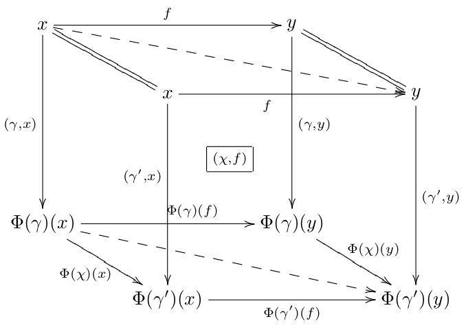
On the other hand, the vertical category has the same objects as , but different morphisms: it’s not hard to see that the vertical category is just the transformation groupoid for the action of the group of -objects on the set of -objects, . Meanwhile, the horizontal morphisms and squares make up the transformation groupoid . These are the object-category and morphism-category of the transpose of the double-category we started with.

We can take this further: if squares aren’t hip enough for you – or if you’re someone who’s happy with 2-categories but finds double categories unfamiliar – the horizontal and vertical categories can be extended to make horizontal and vertical bicategories. They have the same objects and morphisms, but we add new 2-cells which correspond to squares where the boundaries have identity morphisms in the direction we’re not interested in. These two turn out to feel quite different in style.

First, the horizontal bicategory extends by adding 2-morphisms to it, corresponding to morphisms of : roughly, it makes the morphisms of into the objects of a new transformation groupoid, based on the action of the group of automorphisms of the identity in (which ensures the square has identity edges on the sides.) This last point is the only constraint, and it’s not a very strong one since and essentially determine the entire 2-group: the constraint only relates to the structure of .

The constraint for the vertical bicategory is different in flavour because it depends more on the action . Here we are extending a transformation groupoid, . But, for some actions, many morphisms in might just not show up at all. For 1-morphisms , the only 2-morphisms which can appear are those taking to some which has the same effect on as . So, for example, this will look very different if is free (so only automorphisms show up), or a trivial action (so that all morphisms appear).

In the paper, we look at these in the special case of an adjoint action of a 2-group, so you can look there if you’d like a more concrete example of this difference.

Speculative Remarks

The starting point for this was a project (which I talked about a year ago) to do with higher gauge theory – see the last part of the linked post for more detail. The point is that, in gauge theory, one deals with connections on bundles, and morphisms between them called gauge transformations. If one builds a groupoid out of these in a natural way, it turns out to result from the action of a big symmetry group of all gauge transformations on the moduli space of connections.

In higher gauge theory, one deals with connections on gerbes (or higher gerbes – a bundle is essentially a “0-gerbe”). There are now also (2-)morphisms between gauge transformations (and, in higher cases, this continues further), which Roger Picken and I have been calling “gauge modifications”. If we try to repeat the situation for gauge theory, we can construct a 2-groupoid out of these, which expresses this local symmetry. The thing which is different for gerbes (and will continue to get even more different if we move to -gerbes and the corresponding -groupoids) is that this is not the same type of object as a transformation double category.

Now, in our next paper (which this one was written to make possible) we show that the 2-groupoid is actually very intimately related to the transformation double category: that is, the local picture of symmetry for a higher gauge theory is, just as in the lower-dimensional situation, intimately related to a global symmetry of an entire moduli 2-space, i.e. a category. The reason this wasn’t obvious at first is that the moduli space which includes only connections is just the space of objects of this category: the point is that there are really two special kinds of gauge transformations. One should be thought of as the morphisms in the moduli 2-space, and the other as part of the symmetries of that 2-space. The intuition that comes from ordinary gauge theory overlooks this, because the phenomenon doesn’t occur there.

Physically-motivated theories are starting to use these higher-categorical concepts more and more, and symmetry is a crucial idea in physics. What I’ve sketched here is presumably only the start of a pattern in which “symmetry” extends to higher-categorical entities. When we get to 3-groups, our simplifying assumptions that use “strictification” results won’t even be available any more, so we would expect still further new phenomena to show up – but it seems plausible that the tight relation between global and local symmetry will still exist, but in a way that is more subtle, and refines the standard understanding we have of symmetry today.

 

Seminar on the Cobordism Hypothesis and (Infinity,n)-Categories

Well, it’s been a while, but it’s now a new semester here in Hamburg, and I wanted to go back and look at some of what we talked about in last semester’s research seminar. This semester, Susama Agarwala and I are sharing the teaching in a topics class on “Category Theory for Geometry“, in which I’ll be talking about categories of sheaves, and building up the technology for Susama to talk about Voevodsky’s theory of motives (enough to give a starting point to read something like this).

As for last semester’s seminar, one of the two main threads, the one which Alessandro Valentino and I helped to organize, was a look at some of the material needed to approach Jacob Lurie’s paper on the classification of topological quantum field theories. The idea was for the research seminar to present the basic tools that are used in that paper to a larger audience, mostly of graduate students – enough to give a fairly precise statement, and develop the tools needed to follow the proof. (By the way, for a nice and lengthier discussion by Chris Schommer-Pries about this subject, which includes more details on much of what’s in this post, check out this video.)

So: the key result is a slightly generalized form of the Cobordism Hypothesis.

Cobordism Hypothesis

The sort of theory which the paper classifies are those which “extend down to a point”. So what does this mean? A topological field theory can be seen as a sort of “quantum field theory up to homotopy”, which abstract away any geometric information about the underlying space where the fields live – their local degrees of freedom.  We do this by looking only at the classes of fields up to the diffeomorphism symmetries of the space.  The local, geometric, information gets thrown away by taking this quotient of the space of solutions.

In spite of reducing the space of fields this way, we want to capture the intuition that the theory is still somehow “local”, in that we can cut up spaces into parts and make sense of the theory on those parts separately, and determine what it does on a larger space by gluing pieces together, rather than somehow having to take account of the entire space at once, indissolubly. This reasoning should apply to the highest-dimensional space, but also to boundaries, and to any figures we draw on boundaries when cutting them up in turn.

Carrying this on to the logical end point, this means that a topological quantum field theory in the fully extended sense should assign some sort of data to every geometric entity from a zero-dimensional point up to an -dimensional cobordism.  This is all expressed by saying it’s an -functor:

.

Well, once we know what this means, we’ll know (in principle) what a TQFT is.  It’s less important, for the purposes of Lurie’s paper, what is than what is.  The reason is that we want to classify these field theories (i.e. functors).  It will turn out that has the sort of structure that makes it easy to classify the functors out of it into any target -category .  A guess about what kind of structure is actually there was expressed by Baez and Dolan as the Cobordism Hypothesis.  It’s been slightly rephrased from the original form to get a form which has a proof.  The version Lurie proves says:

The -category is equivalent to the free symmetric monoidal -category generated by one fully-dualizable object.

The basic point is that, since is a free structure, the classification means that the extended TQFT’s amount precisely to the choice of a fully-dualizable object of (which includes a choice of a bunch of morphisms exhibiting the “dualizability”). However, to make sense of this, we need to have a suitable idea of an -category, and know what a fully dualizable object is. Let’s begin with the first.

-Categories

In one sense, the Cobordism Hypothesis, which was originally made about -categories at a time when these were only beginning to be defined, could be taken as a criterion for an acceptable definition. That is, it expressed an intuition which was important enough that any definition which wouldn’t allow one to prove the Cobordism Hypothesis in some form ought to be rejected. To really make it work, one had to bring in the “infinity” part of -categories. The point here is that we are talking about category-like structures which have morphisms between objects, 2-morphisms between morphisms, and so on, with -morphisms between -morphisms for every possible degree. The inspiration for this comes from homotopy theory, where one has maps, homotopies of maps, homotopies of homotopies, etc.

Nowadays, there are several possible concrete models for -categories (see this survey article by Julie Bergner for a summary of four of them). They are all equivalent definitions, in a suitable up-to-homotopy way, but for purposes of the proof, Lurie is taking the definition that an -category is an n-fold complete Segal space. One theme that shows up in all the definitions is that of simplicial methods. (In our seminar, we started with a series of two talks introducing the notions of simplicial sets, simplicial objects in a category, and Kan complexes. If you don’t already know this, essentially everything we need is nicely explained in here.)

One of the underlying ideas is that a category can be associated with a simplicial set, its nerve , where the set of -dimensional simplexes is just the set of composable -tuples of morphisms in . If is a groupoid (everything is invertible), then the simplicial set is a Kan complex – it satisfies some filling conditions, which ensure that any morphism has an inverse. Not every Kan complex is the nerve of a groupoid, but one can think of them as weak versions of groupoids – -groupoids, or -categories – where the higher morphisms may not be completely trivial (as with a groupoid), but where at least they’re all invertible. This leads to another desirable feature in any definition of -category, which is the Homotopy Hypothesis: that the -category of -categories, also called -groupoids, should be equivalent (in the same weak sense) to a category of Hausdorff spaces with some other nice properties, which we call for short. This is true of Kan complexes.

Thus, up to homotopy, specifying an -groupoid is the same as specifying a space.

The data which defines a Segal space (which was however first explicitly defined by Charlez Rezk) is a simplicial space : for each , there are spaces , thought of as the space of composable -tuples of morphisms. To keep things tame, we suppose that , the space of objects, is discrete – that is, we have only a set of objects. Being a simplicial space means that the come equipped with a collection of face maps , which we should think of as compositions: to get from an -tuple to an -tuple of morphisms, one can compose two morphisms together at any of positions in the tuple.

One condition which a simplicial space has to satisfy to be a Segal space has to do with the “weakening” which makes a Segal space a weaker notion than just a category lies in the fact that the cannot be arbitrary, but must be homotopy equivalent to the “actual” space of -tuples, which is a strict pullback . That is, in a Segal space, the pullback which defines these tuples for a category is weakened to be a homotopy pullback. Combining this with the various face maps, we therefore get a weakened notion of composition: . Because we start by replacing the space of -tuples with the homotopy-equivalent , the composition rule will only satisfy all the relations which define composition (associativity, for instance) up to homotopy.

To be complete, the Segal space must have a notion of equivalence for which agrees with that for Kan complexes seen as -groupoids. In particular, there is a sub-simplicial object , which we understand to consist of the spaces of invertible -morphisms. Since there should be nothing interesting happening above the top dimension, we ask that, for these spaces, the face and degeneracy maps are all homotopy equivalences: up to homotopy, the space of invertible higher morphisms has no new information.

Then, an -fold complete Segal space is defined recursively, just as one might define -categories (without the infinitely many layers of invertible morphisms “at the top”). In that case, we might say that a double category is just a category internal to : it has a category of objects, and a category of morphims, and the various maps and operations, such as composition, which make up the definition of a category are all defined as functors. That turns out to be the same as a structure with objects, horizontal and vertical morphisms, and square-shaped 2-cells. If we insist that the category of objects is discrete (i.e. really just a set, with no interesting morphisms), then the result amounts to a 2-category. Then we can define a 3-category to be a category internal to (whose 2-category of objects is discrete), and so on. This approach really defines an -fold category (see e.g. Chapter 5 of Cheng and Lauda to see a variation of this approach, due to Tamsamani and Simpson), but imposing the condition that the objects really amount to a set at each step gives exactly the usual intuition of a (strict!) -category.

This is exactly the approach we take with -fold complete Segal spaces, except that some degree of weakness is automatic. Since a C.S.S. is a simplicial object with some properties (we separately define objects of -tuples of morphisms for every , and all the various composition operations), the same recursive approach leads to a definition of an “-fold complete Segal space” as simply a simplicial object in -fold C.S.S.’s (with the same properties), such that the objects form a set. In principle, this gives a big class of “spaces of morphisms” one needs to define – one for every -fold product of simplexes of any dimension – but all those requirements that any space of objects “is just a set” (i.e. is homotopy-equivalent to a discrete set of points) simplifies things a bit.

Cobordism Category as -Category

So how should we think of cobordisms as forming an -category? There are a few stages in making a precise definition, but the basic idea is simple enough. One starts with manifolds and cobordisms embedded in some fixed finite-dimensional vector space , and then takes a limit over all . In each , the coordinates of the factor give ways of cutting the cobordism into pieces, and gluing them back together defines composition in a different direction. Now, this won’t actually produce a complete Segal space: one has to take a certain kind of completion. But the idea is intuitive enough.

We want to define an -fold C.S.S. of cobordisms (and cobordisms between cobordisms, and so on, up to -morphisms). To start with, think of the case : then the space of objects of consists of all embeddings of a -dimensional manifold into . The space of -simplexes (of -tuples of morphisms) consists of all ways of cutting up a -dimensional cobordism embedded in by choosing , where we think of the cobordism having been glued from two pieces, where at the slice , we have the object where the two pieces were composed. (One has to be careful to specify that the Morse function on the cobordisms, got by projection only , has its critical points away from the – the generic case – to make sure that the objects where gluing happens are actual manifolds.)

Now, what about the higher morphisms of the -category? The point is that one needs to have an -groupoid – that is, a space! – of morphisms between two cobordisms and . To make sense of this, we just take the space of diffeomorphisms – not just as a set of morphisms, but including its topology as well. The higher morphisms, therefore, can be thought of precisely as paths, homotopies, homotopies between homotopies, and so on, in these spaces. So the essential difference between the 1-category of cobordisms and the -category is that in the first case, morphisms are diffeomorphism classes of cobordisms, whereas in the latter, the higher morphisms are made precisely of the space of diffeomorphisms which we quotient out by in the first case.

Now, -categories, can have non-invertible morphisms between morphisms all the way up to dimension , after which everything is invertible. An -fold C.S.S. does this by taking the definition of a complete Segal space and copying it inside -fold C.S.S’s: that is, one has an -fold Complete Segal Space of -tuples of morphisms, for each , they form a simplicial object, and so forth.

Now, if we want to build an -category of cobordisms, the idea is the same, except that we have a simplicial object, in a category of simplicial objects, and so on. However, the way to define this is essentially similar. To specify an -fold C.S.S., we have to specify a whole collection of spaces associated to cobordisms equipped with embeddings into . In particular, for each tuple , we have the space of such embeddings, such that for each one has special points along the coordinate axis. These are the ways of breaking down a given cobordism into a composite of pieces. Again, one has to make sure that these critical points of the Morse functions defined by the projections onto these coordinate axes avoid these special which define the manifolds where gluing takes place. The composition maps which make these into a simplical object are quite natural – they just come by deleting special points.

Finally, we take a limit over all (to get around limits to embeddings due to the dimension of ). So we know (at least abstractly) what the -category of cobordisms should be. The cobordism hypothesis claims it is equivalent to one defined in a free, algebraically-flavoured way, namely as the free symmetric monoidal -category on a fully-dualizable object. (That object is “the point” – which, up to the kind of homotopically-flavoured equivalence that matters here, is the only object when our highest-dimensional cobordisms have dimension ).

Dualizability

So what does that mean, a “fully dualizable object”?

First, to get the idea, let’s think of the 1-dimensional example.  Instead of “-category”, we would like to just think of this as a statement about a category.  Then is the 1-category of framed bordisms. For a manifold (or cobordism, which is a manifold with boundary), a framing is a trivialization of the tangent bundle.  That is, it amounts to a choice of isomorphism at each point between the tangent space there and the corresponding .  So the objects of are collections of (signed) points, and the morphisms are equivalence classes of framed 1-dimensional cobordisms.  These amount to oriented 1-manifolds with boundary, where the points (objects) on the boundary are the source and target of the cobordism.

Now we want to classify what TQFT’s live on this category.  These are functors .  We have two generating objects, and , the two signed points.  A TQFT must assign these objects vector spaces, which we’ll call and .  Collections of points get assigned tensor products of all the corresponding vector spaces, since the functor is monoidal, so knowing these two vector spaces determines what does to all objects.

What does do to morphisms?  Well, some generating morphsims of interest are cups and caps: these are lines which connect a positive to a negative point, but thought of as cobordisms taking two points to the empty set, and vice versa.  That is, we have an evaluation:This statement is what is generalized to say that -dimensional TQFT’s are classified by “fully” dualizable objects.

and a coevaluation:

Now, since cobordisms are taken up to equivalence, which in particular includes topological deformations, we get a bunch of relations which these have to satisfy.  The essential one is the “zig-zag” identity, reflecting the fact that a bent line can be straightened out, and we have the same 1-morphism in .  This implies that:

is the same as the identity.  This in turn means that the evaluation and coevaluation maps define a nondegenerate pairing between and .  The fact that this exists means two things.  First, is the dual of : .  Second, this only makes sense if both and its dual are finite dimensional (since the evaluation will just be the trace map, which is not even defined on the identity if is infinite dimensional).

On the other hand, once we know, , this determines up to isomorphism, as well as the evaluation and coevaluation maps.  In fact, this turns out to be enough to specify entirely.  The classification then is: 1-D TQFT’s are classified by finite-dimensional vector spaces .  Crucially, what made finiteness important is the existence of the dual and the (co)evaluation maps which express the duality.

In an -category, to say that an object is “fully dualizable” means more that the object has a dual (which, itself, implies the existence of the morphisms and ). It also means that and have duals themselves – or rather, since we’re talking about morphisms, “adjoints”. This in turn implies the existence of 2-morphisms which are the unit and counit of the adjunctions (the defining properties are essentially the same as those for morphisms which define a dual). In fact, every time we get a morphism of degree less than in this process, “fully dualizable” means that it too must have a dual (i.e. an adjoint).

This does run out eventually, though, since we only require this goes up to dimension : the -morphisms which this forces to exist (quite a few) aren’t required to have duals. This is good, because if they were, since all the higher morphisms available are invertible, this would mean that the dual -morphisms would actually be weak inverses (that is, their composite is isomorphic to the identity)… But that would mean that the dual -morphisms which forced them to exist would also be weak inverses (their composite would be weakly isomorphic to the identity)… and so on! In fact, if the property of “having duals” didn’t stop, then everything would be weakly invertible: we’d actually have a (weak) -groupoid!

Classifying TQFT

So finally, the point of the Cobordism Hypothesis is that a (fully extended) TQFT is a functor out of this into some target -category . There are various options, but whatever we pick, the functor must assign something in to the point, say , and something to each of and , as well as all the higher morphisms which must exist. Then functoriality means that all these images have to again satisfy the properties which make a fully dualizable object. Furthermore, since is the free gadget with all these properties on the single object , this is exactly what it means that is a functor. Saying that is fully dualizable, by implication, includes all the choices of morphisms like etc. which show it as fully dualizable. (Conceivably one could make the same object fully dualizable in more than one way – these would be different functors).

So an extended -dimensional TQFT is exactly the choice of a fully dualizable object , for some -category . This object is “what the TQFT assigns to a point”, but if we understand the structure of the object as a fully dualizable object, then we know what the TQFT assigns to any other manifold of any dimension up to , the highest dimension in the theory. This is how this algebraic characterization of cobordisms helps to classify such theories.

 

Moving to Hamburg; Talk in Brno: 2-Symmetry of Moduli Spaces

Hamburg

Since I moved to Hamburg,   Alessandro Valentino and I have been organizing one series of seminar talks whose goal is to bring people (mostly graduate students, and some postdocs and others) up to speed on the tools used in Jacob Lurie’s big paper on the classification of TQFT and proof of the Cobordism Hypothesis.  This is part of the Forschungsseminar (“research seminar”) for the working groups of Christoph Schweigert, Ingo Runkel, and Christoph Wockel.  First, I gave one introducing myself and what I’ve done on Extended TQFT. In our main series We’ve had a series of four so far – two in which Alessandro outlined a sketch of what Lurie’s result is, and another two by Sebastian Novak and Marc Palm that started catching our audience up on the simplicial methods used in the theory of -categories which it uses.  Coming up in the New Year, Nathan Bowler and I will be talking about first -categories, and then -categories.   I’ll do a few posts summarizing the talks around then.

Some people in the group have done some work on quantum field theories with defects, in relation to which, there’s this workshop coming up here in February!  The idea here is that one could have two regions of space where different field theories apply, which are connected along a boundary. We might imagine these are theories which are different approximations to what’s going on physically, with a different approximation useful in each region.  Whatever the intuition, the regions will be labelled by some category, and boundaries between regions are labelled by functors between categories.  Where different boundary walls meet, one can have natural transformations.  There’s a whole theory of how a 3D TQFT can be associated to modular tensor categories, in sort of the same sense that a 2D TQFT is associated to a Frobenius algebra. This whole program is intimately connected with the idea of “extending” a given TQFT, in the sense that it deals with theories that have inputs which are spaces (or, in the case of defects, sub-spaces of given ones) of many different dimensions.  Lurie’s paper describing the n-dimensional cobordism category, is very much related to the input to a theory like this.

Brno Visit

This time, I’d like to mention something which I began working on with Roger Picken in Lisbon, and talked about for the first time in Brno, Czech Republic, where I was invited to visit at Masaryk University.  I was in Brno for a week or so, and on Thursday, December 13, I gave this talk, called “Higher Gauge Theory and 2-Group Actions”.  But first, some pictures!

This fellow was near the hotel I stayed in:

Since this sculpture is both faceless and hard at work on nonspecific manual labour, I assume he’s a Communist-era artwork, but I don’t really know for sure.

The Christmas market was on in Náměstí Svobody (Freedom Square) in the centre of town.  This four-headed dragon caught my eye:

On the way back from Brno to Hamburg, I met up with my wife to spend a couple of days in Prague.  Here’s the Christmas market in the Old Town Square of Prague:

Anyway, it was a good visit to the Czech Republic.  Now, about the talk!

Moduli Spaces in Higher Gauge Theory

The motivation which I tried to emphasize is to define a specific, concrete situation in which to explore the concept of “2-Symmetry”.  The situation is supposed to be, if not a realistic physical theory, then at least one which has enough physics-like features to give a good proof of concept argument that such higher symmetries should be meaningful in nature.  The idea is that Higher Gauge theory is a field theory which can be understood as one in which the possible (classical) fields on a space/spacetime manifold consist of maps from that space into some target space .  For the topological theory, they are actually just homotopy classes of maps.  This is somewhat related to Sigma models used in theoretical physics, and mathematically to Homotopy Quantum Field Theory, which considers these maps as geometric structure on a manifold.  An HQFT is a functor taking such structured manifolds and cobordisms into Hilbert spaces and linear maps.  In the paper Roger and I are working on, we don’t talk about this stage of the process: we’re just considering how higher-symmetry appears in the moduli spaces for fields of this kind, which we think of in terms of Higher Gauge Theory.

Ordinary topological gauge theory – the study of flat connections on -bundles for some Lie group , can be looked at this way.  The target space is the “classifying space” of the Lie group – homotopy classes of maps in are the same as groupoid homomorphisms in .  Specifically, the pair of functors and relating groupoids and topological spaces are adjoints.  Now, this deals with the situation where is a homotopy 1-type, which is to say that it has a fundamental groupoid , and no other interesting homotopy groups.  To deal with more general target spaces , one should really deal with infinity-groupoids, which can capture the whole homotopy type of – in particular, all its higher homotopy groups at once (and various relations between them).  What we’re talking about in this paper is exactly one step in that direction: we deal with 2-groupoids.

We can think of this in terms of maps into a target space which is a 2-type, with nontrivial fundamental groupoid , but also interesting second homotopy group (and nothing higher).  These fit together to make a 2-groupoid , which is a 2-group if is connected.  The idea is that is the classifying space of some 2-group , which plays the role of the Lie group in gauge theory.  It is the “gauge 2-group”.  Homotopy classes of maps into correspond to flat connections in this 2-group.

For practical purposes, we use the fact that there are several equivalent ways of describing 2-groups.  Two very directly equivalent ways to define them are as group objects internal to , or as categories internal to – which have a group of objects and a group of morphisms, and group homomorphisms that define source, target, composition, and so on.  This second way is fairly close to the equivalent formulation as crossed modules .  The definition is in the slides, but essentially the point is that is the group of objects, and with the action , one gets the semidirect product which is the group of morphisms.  The map makes it possible to speak of and acting on each other, and that these actions “look like conjugation” (the precise meaning of which is in the defining properties of the crossed module).

The reason for looking at the crossed-module formulation is that it then becomes fairly easy to understand the geometric nature of the fields we’re talking about.  In ordinary gauge theory, a connection can be described locally as a 1-form with values in , the Lie algebra of .  Integrating such forms along curves gives another way to describe the connection, in terms of a rule assigning to every curve a holonomy valued in which describes how to transport something (generally, a fibre of a bundle) along the curve.  It’s somewhat nontrivial to say how this relates to the classic definition of a connection on a bundle, which can be described locally on “patches” of the manifold via 1-forms together with gluing functions where patches overlap.  The resulting categories are equivalent, though.

In higher gauge theory, we take a similar view. There is a local view of “connections on gerbes“, described by forms and gluing functions (the main difference in higher gauge theory is that the gluing functions related to higher cohomology).  But we will take the equivalent point of view where the connection is described by -valued holonomies along paths, and -valued holonomies over surfaces, for a crossed module , which satisfy some flatness conditions.  These amount to 2-functors of 2-categories .

The moduli space of all such 2-connections is only part of the story.  2-functors are related by natural transformations, which are in turn related by “modifications”.  In gauge theory, the natural transformations are called “gauge transformations”, and though the term doesn’t seem to be in common use, the obvious term for the next layer would be “gauge modifications”. It is possible to assemble a 2-groupoid , whose space of objects is exactly the moduli space of 2-connections, and whose 1- and 2-morphisms are exactly these gauge transformations and modifications.  So the question is, what is the meaning of the extra information contained in the 2-groupoid which doesn’t appear in the moduli space itself?

Our claim is that this information expresses how the moduli space carries “higher symmetry”.

2-Group Actions and the Transformation Double Category

What would it mean to say that something exhibits “higher” symmetry? A rudimentary way to formalize the intuition of “symmetry” is to say that there is a group (of “symmetries”) which acts on some object. One could get more subtle, but this should be enough to begin with. We already noted that “higher” gauge theory uses 2-groups (and beyond into -groups) in the place of ordinary groups.  So in this context, the natural way to interpret it is by saying that there is an action of a 2-group on something.

Just as there are several equivalent ways to define a 2-group, there are different ways to say what it means for it to have an action on something.  One definition of a 2-group is to say that it’s a 2-category with one object and all morphisms and 2-morphisms invertible.  This definition makes it clear that a 2-group has to act on an object of some 2-category . For our purposes, just as we normally think of group actions on sets, we will focus on 2-group actions on categories, so that is the 2-category of interest. Then an action is just a map:

The unique object of – let’s call it , gets taken to some object .  This object is the thing being “acted on” by .  The existence of the action implies that there are automorphisms for every morphism in (which correspond to the elements of the group of the crossed module).  This would be enough to describe ordinary symmetry, but the higher symmetry is also expressed in the images of 2-morphisms , which we might call 2-symmetries relating 1-symmetries.

What we want to do in our paper, which the talk summarizes, is to show how this sort of 2-group action gives rise to a 2-groupoid (actually, just a 2-category when the being acted on is a general category).  Then we claim that the 2-groupoid of connections can be seen as one that shows up in exactly this way.  (In the following, I have to give some credit to Dany Majard for talking this out and helping to find a better formalism.)

To make sense of this, we use the fact that there is a diagrammatic way to describe the transformation groupoid associated to the action of a group on a set .  The set of morphisms is built as a pullback of the action map, .

This means that morphisms are pairs , thought of as going from to .  The rule for composing these is another pullback.  The diagram which shows how it’s done appears in the slides.  The whole construction ends up giving a cubical diagram in , whose top and bottom faces are mere commuting diagrams, and whose four other faces are all pullback squares.

To construct a 2-category from a 2-group action is similar. For now we assume that the 2-group action is strict (rather than being given by a weak 2-functor).  In this case, it’s enough to think of our 2-group not as a 2-category, but as a group-object in – the same way that a 1-group, as well as being a category, can be seen as a group object in .  The set of objects of this category is the group of morphisms of the 2-category, and the morphisms make up the group of 2-morphisms.  Being a group object is the same as having all the extra structure making up a 2-group.

To describe a strict action of such a on , we just reproduce in the diagram that defines an action in :

The fact that is an action just means this commutes. In principle, we could define a weak action, which would mean that this commutes up to isomorphism, but we won’t be looking at that here.

Constructing the same diagram which describes the structure of a transformation groupoid (p29 in the slides for the talk), we get a structure with a “category of objects” and a “category of morphisms”.  The construction in gives us directly a set of morphisms, while itself is the set of objects. Similarly, in , the category of objects is just , while the construction gives a category of morphisms.

The two together make a category internal to , which is to say a double category.  By analogy with , we call this double category .

We take as the category of objects, as the “horizontal category”, whose morphisms are the horizontal arrows of the double category. The category of morphisms of shows up by letting its objects be the vertical arrows of the double category, and its morphisms be the squares.  These look like this:

The vertical arrows are given by pairs of objects , and just like the transformation 1-groupoid, each corresponds to the fact that the action of takes to . Each square (morphism in the category of morphisms) is given by a pair of morphisms, one from (given by an element in ), and one from .

The horizontal arrow on the bottom of this square is:

The fact that these are equal is exactly the fact that is a natural transformation.

The double category turns out to have a very natural example which occurs in higher gauge theory.

Higher Symmetry of the Moduli Space

The point of the talk is to show how the 2-groupoid of connections, previously described as , can be seen as coming from a 2-group action on a category – the objects of this category being exactly the connections. In the slides above, for various reasons, we did this in a discretized setting – a manifold with a decomposition into cells. This is useful for writing things down explicitly, but not essential to the idea behind the 2-symmetry of the moduli space.

The point is that there is a category we call , whose objects are the connections: these assign -holonomies to edges of our discretization (in general, to paths), and -holonomies to 2D faces. (Without discretization, one would describe these in terms of -valued 1-forms and -valued 2-forms.)

The morphisms of are one type of “gauge transformation”: namely, those which assign -holonomies to edges. (Or: -valued 1-forms). They affect the edge holonomies of a connection just like a 2-morphism in .  Face holonomies are affected by the -value that comes from the boundary of the face.

What’s physically significant here is that both objects and morphisms of describe nonlocal geometric information.  They describe holonomies over edges and surfaces: not what happens at a point.  The “2-group of gauge transformations”, which we call , on the other hand, is purely about local transformations.  If is the vertex set of the discretized manifold, then : one copy of the gauge 2-group at each vertex.  (Keeping this finite dimensional and avoiding technical details was one main reason we chose to use a discretization.  In principle, one could also talk about the 2-group of -valued functions, whose objects and morphisms, thinking of it as a group object in , are functions valued in morphisms of .)

Now, the way acts on is essentially by conjugation: edge holonomies are affected by pre- and post-multiplication by the values at the two vertices on the edge – whether objects or morphisms of .  (Face holonomies are unaffected).  There are details about this in the slides, but the important thing is that this is a 2-group of purely local changes.  The objects of are gauge transformations of this other type.  In a continuous setting, they would be described by -valued functions.  The morphisms are gauge modifications, and could be described by -valued functions.

The main conceptual point here is that we have really distinguished between two kinds of gauge transformation, which are the horizontal and vertical arrows of the double category .  This expresses the 2-symmetry by moving some gauge transformations into the category of connections, and others into the 2-group which acts on it.  But physically, we would like to say that both are “gauge transformations”.  So one way to do this is to “collapse” the double category to a bicategory: just formally allow horizontal and vertical arrows to compose, so that there is only one kind of arrow.  Squares become 2-cells.

So then if we collapse the double category expressing our 2-symmetry relation this way, the result is exactly equivalent to the functor category way of describing connections.  (The morphisms will all be invertible because is a groupoid and is a 2-group).

I’m interested in this kind of geometrical example partly because it gives a good way to visualize something new happening here.  There appears to be some natural 2-symmetry on this space of fields, which is fairly easy to see geometrically, and distinguishes in a fundamental way between two types of gauge transformation.  This sort of phenomenon doesn’t occur in the world of – a set has no morphisms, after all, so the transformation groupoid for a group action on it is much simpler.

In broad terms, this means that 2-symmetry has qualitatively new features that familiar old 1-symmetry doesn’t have.  Higher categorical versions – -groups acting on -groupoids, as might show up in more complicated HQFT – will certainly be even more complicated.  The 2-categorical version is just the first non-trivial situation where this happens, so it gives a nice starting point to understand what’s new in higher symmetry that we didn’t already know.

 

Higher Structures in China

Since the last post, I’ve been busily attending some conferences, as well as moving to my new job at the University of Hamburg, in the Graduiertenkolleg 1670, “Mathematics Inspired by String Theory and Quantum Field Theory”.  The week before I started, I was already here in Hamburg, at the conference they were organizing “New Perspectives in Topological Quantum Field Theory“.  But since I last posted, I was also at the 20th Oporto Meeting on Geometry, Topology, and Physics, as well as the third Higher Structures in China workshop, at Jilin University in Changchun.  Right now, I’d like to say a few things about some of the highlights of that workshop.

Higher Structures in China III

So last year I had a bunch of discussions I had with Chenchang Zhu and Weiwei Pan, who at the time were both in Göttingen, about my work with Jamie Vicary, which I wrote about last time when the paper was posted to the arXiv.  In that, we showed how the Baez-Dolan groupoidification of the Heisenberg algebra can be seen as a representation of Khovanov’s categorification.  Chenchang and Weiwei and I had been talking about how these ideas might extend to other examples, in particular to give nice groupoidifications of categorified Lie algebras and quantum groups.

That is still under development, but I was invited to give a couple of talks on the subject at the workshop.  It was a long trip: from Lisbon, the farthest-west of the main cities of (continental) Eurasia all the way to one of the furthest-East.   (Not quite the furthest, but Changchun is in the northeast of China, just a few hours north of Korea, and it took just about exactly 24 hours including stopovers to get there).  It was a long way to go for a three day workshop, but as there were also three days of a big excursion to Changbai Mountain, just on the border with North Korea, for hiking and general touring around.  So that was a sort of holiday, with 11 other mathematicians.  Here is me with Dany Majard, in a national park along the way to the mountains:

Here’s me with Alex Hoffnung, on Changbai Mountain (in the background is China):

And finally, here’s me a little to the left of the previous picture, where you can see into the volcanic crater.  The lake at the bottom is cut out of the picture, but you can see the crater rim, of which this particular part is in North Korea, as seen from China:

Well, that was fun!

Anyway, the format of the workshop involved some talks from foreigners and some from locals, with a fairly big local audience including a good many graduate students from Jilin University.  So they got a chance to see some new work being done elsewhere – mostly in categorification of one kind or another.  We got a chance to see a little of what’s being done in China, although not as much as we might have. I gather that not much is being done yet that fit the theme of the workshop, which was part of the reason to organize the workshop, and especially for having a session aimed specially at the graduate students.

Categorified Algebra

This is a sort of broad term, but certainly would include my own talk.  The essential point is to show how the groupoidification of the Heisenberg algebra is a representation of Khovanov’s categorification of the same algebra, in a particular 2-category.  The emphasis here is on the fact that it’s a representation in a 2-category whose objects are groupoids, but whose morphisms aren’t just functors, but spans of functors – that is, composites of functors and co-functors.  This is a pretty conservative weakening of “representations on categories” – but it lets one build really simple combinatorial examples.  I’ve discussed this general subject in recent posts, so I won’t elaborate too much.  The lecture notes are here, if you like, though – they have more detail than my previous post, but are less technical than the paper with Jamie Vicary.

Aaron Lauda gave a nice introduction to the program of categorifying quantum groups, mainly through the example of the special case , somewhat along the same lines as in his introductory paper on the subject.  The story which gives the motivation is nice: one has knot invariants such as the Jones polynomial, based on representations of groups and quantum groups.  The Jones polynomial can be categorified to give Khovanov homology (which assigns a complex to a knot, whose graded Euler characteristic is the Jones polynomial) – but also assigns maps of complexes to cobordisms of knots.  One then wants to categorify the representation theory behind it – to describe actions of, for instance, quantum on categories.  This starting point is nice, because it can work by just mimicking the construction of and representations in terms of weight spaces: one gets categories which correspond to the “weight spaces” (usually just vector spaces), and the and operators give functors between them, and so forth.

Finding examples of categories and functors with this structure, and satisfying the right relations, gives “categorified representations” of the algebra – the monoidal categories of diagrams which are the “categorifications of the algebra” then are seen as the abstraction of exactly which relations these are supposed to satisfy.  One such example involves flag varieties.  A flag, as one might eventually guess from the name, is a nested collection of subspaces in some -dimensional space.  A simple example is the Grassmannian , which is the space of all 1-dimensional subspaces of (i.e. the projective space ), which is of course an algebraic variety.  Likewise, , the space of all -dimensional subspaces of is a variety.  The flag variety consists of all pairs , of a -dimensional subspace of , inside a -dimensional subspace (the case calls to mind the reason for the name: a plane intersecting a given line resembles a flag stuck to a flagpole).  This collection is again a variety.  One can go all the way up to the variety of “complete flags”, (where is -dimenisonal), any point of which picks out a subspace of each dimension, each inside the next.

The way this relates to representations is by way of geometric representation theory. One can see those flag varieties of the form as relating the Grassmanians: there are projections and , which act by just ignoring one or the other of the two subspaces of a flag.  This pair of maps, by way of pulling-back and pushing-forward functions, gives maps between the cohomology rings of these spaces.  So one gets a sequence , and maps between the adjacent ones.  This becomes a representation of the Lie algebra.  Categorifying this, one replaces the cohomology rings with derived categories of sheaves on the flag varieties – then the same sort of “pull-push” operation through (derived categories of sheaves on) the flag varieties defines functors between those categories.  So one gets a categorified representation.

Heather Russell‘s talk, based on this paper with Aaron Lauda, built on the idea that categorified algebras were motivated by Khovanov homology.  The point is that there are really two different kinds of Khovanov homology – the usual kind, and an Odd Khovanov Homology, which is mainly different in that the role played in Khovanov homology by a symmetric algebra is instead played by an exterior (antisymmetric) algebra.  The two look the same over a field of characteristic 2, but otherwise different.  The idea is then that there should be “odd” versions of various structures that show up in the categorifications of (and other algebras) mentioned above.

One example is the fact that, in the “even” form of those categorifications, there is a natural action of the Nil Hecke algebra on composites of the generators.  This is an algebra which can be seen to act on the space of polynomials in commuting variables, , generated by the multiplication operators , and the “divided difference operators” based on the swapping of two adjacent variables.  The Hecke algebra is defined in terms of “swap” generators, which satisfy some -deformed variation of the relations that define the symmetric group (and hence its group algebra).   The Nil Hecke algebra is so called since the “swap” (i.e. the divided difference) is nilpotent: the square of the swap is zero.  The way this acts on the objects of the diagrammatic category is reflected by morphisms drawn as crossings of strands, which are then formally forced to satisfy the relations of the Nil Hecke algebra.

The ODD Nil Hecke algebra, on the other hand, is an analogue of this, but the are anti-commuting, and one has different relations satisfied by the generators (they differ by a sign, because of the anti-commutation).  This sort of “oddification” is then supposed to happen all over.  The main point of the talk was to to describe the “odd” version of the categorified representation defined using flag varieties.  Then the odd Nil Hecke algebra acts on that, analogously to the even case above.

Marco Mackaay gave a couple of talks about the web algebra, describing the results of this paper with Weiwei Pan and Daniel Tubbenhauer.  This is the analog of the above, for , describing a diagram calculus which accounts for representations of the quantum group.  The “web algebra” was introduced by Greg Kuperberg – it’s an algebra built from diagrams which can now include some trivalent vertices, along with rules imposing relations on these.  When categorifying, one gets a calculus of “foams” between such diagrams.  Since this is obviously fairly diagram-heavy, I won’t try here to reproduce what’s in the paper – but an important part of is the correspondence between webs and Young Tableaux, since these are labels in the representation theory of the quantum group – so there is some interesting combinatorics here as well.

Algebraic Structures

Some of the talks were about structures in algebra in a more conventional sense.

Jiang-Hua Lu: On a class of iterated Poisson polynomial algebras.  The starting point of this talk was to look at Poisson brackets on certain spaces and see that they can be found in terms of “semiclassical limits” of some associative product.  That is, the associative product of two elements gives a power series in some parameter (which one should think of as something like Planck’s constant in a quantum setting).  The “classical” limit is the constant term of the power series, and the “semiclassical” limit is the first-order term.  This gives a Poisson bracket (or rather, the commutator of the associative product does).  In the examples, the spaces where these things are defined are all spaces of polynomials (which makes a lot of explicit computer-driven calculations more convenient). The talk gives a way of constructing a big class of Poisson brackets (having some nice properties: they are “iterated Poisson brackets”) coming from quantum groups as semiclassical limits.  The construction uses words in the generating reflections for the Weyl group of a Lie group .

Li Guo: Successors and Duplicators of Operads – first described a whole range of different algebra-like structures which have come up in various settings, from physics and dynamical systems, through quantum field theory, to Hopf algebras, combinatorics, and so on.  Each of them is some sort of set (or vector space, etc.) with some number of operations satisfying some conditions – in some cases, lots of operations, and even more conditions.  In the slides you can find several examples – pre-Lie and post-Lie algebras, dendriform algebras, quadri- and octo-algebras, etc. etc.  Taken as a big pile of definitions of complicated structures, this seems like a terrible mess.  The point of the talk is to point out that it’s less messy than it appears: first, each definition of an algebra-like structure comes from an operad, which is a formal way of summing up a collection of operations with various “arities” (number of inputs), and relations that have to hold.  The second point is that there are some operations, “successor” and “duplicator”, which take one operad and give another, and that many of these complicated structures can be generated from simple structures by just these two operations.  The “successor” operation for an operad introduces a new product related to old ones – for example, the way one can get a Lie bracket from an associative product by taking the commutator.  The “duplicator” operation takes existing products and introduces two new products, whose sum is the previous one, and which satisfy various nice relations.  Combining these two operations in various ways to various starting points yields up a plethora of apparently complicated structures.

Dany Majard gave a talk about algebraic structures which are related to double groupoids, namely double categories where all the morphisms are invertible.  The first part just defined double categories: graphically, one has horizontal and vertical 1-morphisms, and square 2-morphsims, which compose in both directions.  Then there are several special degenerate cases, in the same way that categories have as degenerate cases (a) sets, seen as categories with only identity morphisms, and (b) monoids, seen as one-object categories.  Double categories have ordinary categories (and hence monoids and sets) as degenerate cases.  Other degenerate cases are 2-categories (horizontal and vertical morphisms are the same thing), and therefore their own special cases, monoidal categories and symmetric monoids.  There is also the special degenerate case of a double monoid (and the extra-special case of a double group).  (The slides have nice pictures showing how they’re all degenerate cases).  Dany then talked about some structure of double group(oids) – and gave a list of properties for double groupoids, (such as being “slim” – having at most one 2-cell per boundary configuration – as well as two others) which ensure that they’re equivalent to the semidirect product of an abelian group with the “bicrossed product”  of two groups and (each of which has to act on the other for this to make sense).  He gave the example of the Poincare double group, which breaks down as a triple bicrossed product by the Iwasawa decomposition:

( is certain group of matrices).  So there’s a unique double group which corresponds to it – it has squares labelled by , and the horizontial and vertical morphisms by elements of and respectively.  Dany finished by explaining that there are higher-dimensional analogs of all this – -tuple categories can be defined recursively by internalization (“internal categories in -tuple-Cat”).  There are somewhat more sophisticated versions of the same kind of structure, and finally leading up to a special class of -tuple groups.  The analogous theorem says that a special class of them is just the same as the semidirect product of an abelian group with an -fold iterated bicrossed product of groups.

Also in this category, Alex Hoffnung talked about deformation of formal group laws (based on this paper with various collaborators).  FGL’s are are structures with an algebraic operation which satisfies axioms similar to a group, but which can be expressed in terms of power series.  (So, in particular they have an underlying ring, for this to make sense).  In particular, the talk was about formal group algebras – essentially, parametrized deformations of group algebras – and in particular for Hecke Algebras.  Unfortunately, my notes on this talk are mangled, so I’ll just refer to the paper.

Physics

I’m using the subject-header “physics” to refer to those talks which are most directly inspired by physical ideas, though in fact the talks themselves were mathematical in nature.

Fei Han gave a series of overview talks intorducing “Equivariant Cohomology via Gauged Supersymmetric Field Theory”, explaining the Stolz-Teichner program.  There is more, using tools from differential geometry and cohomology to dig into these theories, but for now a summary will do.  Essentially, the point is that one can look at “fields” as sections of various bundles on manifolds, and these fields are related to cohomology theories.  For instance, the usual cohomology of a space is a quotient of the space of closed forms (so the cohomology, , is a quotient of the space of closed -forms – the quotient being that forms differing by a coboundary are considered the same).  There’s a similar construction for the -theory , which can be modelled as a quotient of the space of vector bundles over .  Fei Han mentioned topological modular forms, modelled by a quotient of the space of “Fredholm bundles” – bundles of Banach spaces with a Fredholm operator around.

The first two of these examples are known to be related to certain supersymmetric topological quantum field theories.  Now, a TFT is a functor into some kind of vector spaces from a category of -dimensional manifolds and -dimensional cobordisms

Intuitively, it gives a vector space of possible fields on the given space and a linear map on a given spacetime.  A supersymmetric field theory is likewise a functor, but one changes the category of “spacetimes” to have both bosonic and fermionic dimension.  A normal smooth manifold is a ringed space , since it comes equipped with a sheaf of rings (each open set has an associated ring of smooth functions, and these glue together nicely).  Supersymmetric theories work with manifolds which change this sheaf – so a -dimensional space has the sheaf of rings where one introduces some new antisymmetric coordinate functions , the “fermionic dimensions”:

Then a supersymmetric TFT is a functor:

(where is the category of supersymmetric topological vector spaces – defined similarly).  The connection to cohomology theories is that the classes of such field theories, up to a notion of equivalence called “concordance”, are classified by various cohomology theories.  Ordinary cohomology corresponds then to -dimensional extended TFT (that is, with 0 bosonic and 1 fermionic dimension), and -theory to a -dimensional extended TFT.  The Stoltz-Teichner Conjecture is that the third example (topological modular forms) is related in the same way to a -dimensional extended TFT – so these are the start of a series of cohomology theories related to various-dimension TFT’s.

Last but not least, Chris Rogers spoke about his ideas on “Higher Geometric Quantization”, on which he’s written a number of papers.  This is intended as a sort of categorification of the usual ways of quantizing symplectic manifolds.  I am still trying to catch up on some of the geometry This is rooted in some ideas that have been discussed by Brylinski, for example.  Roughly, the message here is that “categorification” of a space can be thought of as a way of acting on the loop space of a space.  The point is that, if points in a space are objects and paths are morphisms, then a loop space shifts things by one categorical level: its points are loops in , and its paths are therefore certain 2-morphisms of .  In particular, there is a parallel to the fact that a bundle with connection on a loop space can be thought of as a gerbe on the base space.  Intuitively, one can “parallel transport” things along a path in the loop space, which is a surface given by a path of loops in the original space.  The local description of this situation says that a 1-form (which can give transport along a curve, by integration) on the loop space is associated with a 2-form (giving transport along a surface) on the original space.

Then the idea is that geometric quantization of loop spaces is a sort of higher version of quantization of the original space. This “higher” version is associated with a form of higher degree than the symplectic (2-)form used in geometric quantization of .   The general notion of n-plectic geometry, where the usual symplectic geometry is the case , involves a -form analogous to the usual symplectic form.  Now, there’s a lot more to say here than I properly understand, much less can summarize in a couple of paragraphs.  But the main theorem of the talk gives a relation between n-plectic manifolds (i.e. ones endowed with the right kind of form) and Lie n-algebras built from the complex of forms on the manifold.  An important example (a theorem of Chris’ and John Baez) is that one has a natural example of a 2-plectic manifold in any compact simple Lie group together with a 3-form naturally constructed from its Maurer-Cartan form.

At any rate, this workshop had a great proportion of interesting talks, and overall, including the chance to see a little more of China, was a great experience!

 

Two Workshops on Representations and Categories – Part I

So I’ve been travelling a lot in the last month, spending more than half of it outside Portugal. I was in Ottawa, Canada for a Fields Institute workshop, “Categorical Methods in Representation Theory“. Then a little later I was in Erlangen, Germany for one called “Categorical and Representation-Theoretic Methods in Quantum Geometry and CFT“. Despite the similar-sounding titles, these were on fairly different themes, though Marco Mackaay was at both, talking about categorifying the -Schur algebra by diagrams.  I’ll describe the meetings, but for now I’ll start with the first.  Next post will be a summary of the second.

The Ottawa meeting was organized by Alistair Savage, and Alex Hoffnung (like me, a former student of John Baez). Alistair gave a talk here at IST over the summer about a -deformation of Khovanov’s categorification of the Heisenberg Algebra I discussed in an earlier entry. A lot of the discussion at the workshop was based on the Khovanov-Lauda program, which began with categorifying quantum version of the classical Lie groups, and is now making lots of progress in the categorification of algebras, representation theory, and so on.

The point of this program is to describe “categorifications” of particular algebras. This means finding monoidal categories with the property that when you take the Grothendieck ring (the ring of isomorphism classes, with a multiplication given by the monoidal structure), you get back the integral form of some algebra. (And then recover the original by taking the tensor over with ). The key thing is how to represent the algebra by generators and relations. Since free monoidal categories with various sorts of structures can be presented as categories of string diagrams, it shouldn’t be surprising that the categories used tend to have objects that are sequences (i.e. monoidal products) of dots with various sorts of labelling data, and morphisms which are string diagrams that carry those labels on strands (actually, usually they’re linear combinations of such diagrams, so everything is enriched in vector spaces). Then one imposes relations on the “free” data given this way, by saying that the diagrams are considered the same morphism if they agree up to some local moves. The whole problem then is to find the right generators (labelling data) and relations (local moves). The result will be a categorification of a given presentation of the algebra you want.

So for instance, I was interested in Sabin Cautis and Anthony Licata‘s talks connected with this paper, “Heisenberg Categorification And Hilbert Schemes”. This is connected with a generalization of Khovanov’s categorification linked above, to include a variety of other algebras which are given a similar name. The point is that there’s such a “Heisenberg algebra” associated to different subgroups , which in turn are classified by Dynkin diagrams. The vertices of these Dynkin diagrams correspond to some generators of the Heisenberg algebra, and one can modify Khovanov’s categorification by having strands in the diagram calculus be labelled by these vertices. Rules for local moves involving strands with different labels will be governed by the edges of the Dynkin diagram. Their paper goes on to describe how to represent these categorifications on certain categories of Hilbert schemes.

Along the same lines, Aaron Lauda gave a talk on the categorification of the NilHecke algebra. This is defined as a subalgebra of endomorphisms of , generated by multiplications (by the ) and the divided difference operators . There are different from the usual derivative operators: in place of the differences between values of a single variable, they measure how a function behaves under the operation which switches variables and (that is, the reflection in the hyperplane where ). The point is that just like differentiation, this operator – together with multiplication – generates an algebra in . Aaron described how to categorify this presentation of the NilHecke algebra with a string-diagram calculus.

So anyway, there were a number of talks about the explosion of work within this general program – for instance, Marco Mackaay’s which I mentioned, as well as that of Pedro Vaz about the same project. One aspect of this program is that the relatively free “string diagram categories” are sometimes replaced with categories where the objects are bimodules and morphisms are bimodule homomorphisms. Making the relationship precise is then a matter of proving these satisfy exactly the relations on a “free” category which one wants, but sometimes they’re a good setting to prove one has a nice categorification. Thus, Ben Elias and Geordie Williamson gave two parts of one talk about “Soergel Bimodules and Kazhdan-Lusztig Theory” (see a blog post by Ben Webster which gives a brief intro to this notion, including pointing out that Soergel bimodules give a categorification of the Hecke algebra).

One of the reasons for doing this sort of thing is that one gets invariants for manifolds from algebras – in particular, things like the Jones polynomial, which is related to the Temperley-Lieb algebra. A categorification of it is Khovanov homology (which gives, for a manifold, a complex, with the property that the graded Euler characteristic of the complex is the Jones polynomial). The point here is that categorifying the algebra lets you raise the dimension of the kind of manifold your invariants are defined on.

So, for instance, Scott Morrison described “Invariants of 4-Manifolds from Khonanov Homology“.  This was based on a generalization of the relationship between TQFT’s and planar algebras.  The point is, planar algebras are described by the composition of diagrams of the following form: a big circle, containing some number of small circles.  The boundaries of each circle are labelled by some number of marked points, and the space between carries curves which connect these marked points in some way.  One composes these diagrams by gluing big circles into smaller circles (there’s some further discussion here including a picture, and much more in this book here).  Scott Morrison described these diagrams as “spaghetti and meatball” diagrams.  Planar algebras show up by associating a vector spaces to “the” circle with marked points, and linear maps to each way (up to isotopy) of filling in edges between such circles.  One can think of the circles and marked-disks as a marked-cobordism category, and so a functorial way of making these assignments is something like a TQFT.  It also gives lots of vector spaces and lots of linear maps that fit together in a particular way described by this category of marked cobordisms, which is what a “planar algebra” actually consists of.  Clearly, these planar algebras can be used to get some manifold invariants – namely the “TQFT” that corresponds to them.

Scott Morrison’s talk described how to get invariants of 4-dimensional manifolds in a similar way by boosting (almost) everything in this story by 2 dimensions.  You start with a 4-ball, whose boundary is a 3-sphere, and excise some number of 4-balls (with 3-sphere boundaries) from the interior.  Then let these 3D boundaries be “marked” with 1-D embedded links (think “knots” if you like).  These 3-spheres with embedded links are the objects in a category.  The morphisms are 4-balls which connect them, containing 2D knotted surfaces which happen to intersect the boundaries exactly at their embedded links.  By analogy with the image of “spaghetti and meatballs”, where the spaghetti is a collection of 1D marked curves, Morrison calls these 4-manifolds with embedded 2D surfaces “lasagna diagrams” (which generalizes to the less evocative case of “ pasta diagrams”, where we’ve just mentioned the and cases, with -dimensional “pasta” embedded in -dimensional balls).  Then the point is that one can compose these pasta diagrams by gluing the 4-balls along these marked boundaries.  One then gets manifold invariants from these sorts of diagrams by using Khovanov homology, which assigns to

Ben Webster talked about categorification of Lie algebra representations, in a talk called “Categorification, Lie Algebras and Topology“. This is also part of categorifying manifold invariants, since the Reshitikhin-Turaev Invariants are based on some monoidal category, which in this case is the category of representations of some algebra.  Categorifying this to a 2-category gives higher-dimensional equivalents of the RT invariants.  The idea (which you can check out in those slides) is that this comes down to describing the analog of the “highest-weight” representations for some Lie algebra you’ve already categorified.

The Lie theory point here, you might remember, is that representations of Lie algebras can be analyzed by decomposing them into “weight spaces” , associated to weights (where is the base field, which we can generally assume is ).  Weights turn Lie algebra elements into scalars, then.  So weight spaces generalize eigenspaces, in that acting by any element on a “weight vector” amounts to multiplying by .  (So that is an eigenvector for each , but the eigenvalue depends on , and is given by the weight.)  A weight can be the “highest” with respect to a natural order that can be put on weights ( if the difference is a nonnegative combination of simple weights).  Then a “highest weight representation” is one which is generated under the action of by a single weight vector , the “highest weight vector”.

The point of the categorification is to describe the representation in the same terms.  First, we introduce a special strand (which Ben Webster draws as a red strand) which represents the highest weight vector.  Then we say that the category that stands in for the highest weight representation is just what we get by starting with this red strand, and putting all the various string diagrams of the categorification of next to it.  One can then go on to talk about tensor products of these representations, where objects are found by amalgamating several such diagrams (with several red strands) together.  And so on.  These categorified representations are then supposed to be usable to give higher-dimensional manifold invariants.

Now, the flip side of higher categories that reproduce ordinary representation theory would be the representation theory of higher categories in their natural habitat, so to speak. Presumably there should be a fairly uniform picture where categorifications of normal representation theory will be special cases of this. Vlodymyr Mazorchuk gave an interesting talk called 2-representations of finitary 2-categories.  He gave an example of one of the 2-categories that shows up a lot in these Khovanov-Lauda categorifications, the 2-category of Soergel Bimodules mentioned above.  This has one object, which we can think of as a category of modules over the algebra (where I  is some ideal of homogeneous symmetric polynomials).  The morphisms are endofunctors of this category, which all amount to tensoring with certain bimodules – the irreducible ones being the Soergel bimodules.  The point of the talk was to explain the representations of 2-categories – that is, 2-functors from into some “classical” 2-category.  Examples would be 2-categories like “2-vector spaces”, or variants on it.  The examples he gave: (1) [small fully additive -linear categories], (2) the full subcategory of it with finitely many indecomposible elements, (3) [categories equivalent to module categories of finite dimensional associative -algebras].  All of these have some claim to be a 2-categorical analog of [vector spaces].  In general, Mazorchuk allowed representations of “FIAT” categories: Finitary (Two-)categories with Involutions and Adjunctions.

Part of the process involved getting a “multisemigroup” from such categories: a set with an operation which takes pairs of elements, and returns a subset of , satisfying some natural associativity condition.  (Semigroups are the case where the subset contains just one element – groups are the case where furthermore the operation is invertible).  The idea is that FIAT categories have some set of generators – indecomposable 1-morphisms – and that the multisemigroup describes which indecomposables show up in a composite.  (If we think of the 2-category as a monoidal category, this is like talking about a decomposition of a tensor product of objects).  So, for instance, for the 2-category that comes from the monoidal category of modules, we get the semigroup of nonnegative integers.  For the Soergel bimodule 2-category, we get the symmetric group.  This sort of thing helps characterize when two objects are equivalent, and in turn helps describe 2-representations up to some equivalence.  (You can find much more detail behind the link above.)

On the more classical representation-theoretic side of things, Joel Kamnitzer gave a talk called “Spiders and Buildings”, which was concerned with some geometric and combinatorial constructions in representation theory.  These involved certain trivalent planar graphs, called “webs”, whose edges carry labels between 1 and .  They’re embedded in a disk, and the outgoing edges, with labels determine a representation space for a group , say , namely the tensor product of a bunch of wedge products, , where acts on as usual.  Then a web determines an invariant vector in this space.  This comes about by having invariant vectors for each vertex (the basic case where ), and tensoring them together.  But the point is to interpret this construction geometrically.  This was a bit outside my grasp, since it involves the Langlands program and the geometric Satake correspondence, neither of which I know much of anything about, but which give geometric/topological ways of constructing representation categories.  One thing I did pick up is that it uses the “Langlands dual group” of to get a certain metric space called .  Then there’s a correspondence between the category of representations of and the category of (perverse, constructible) sheaves on this space.  This correspondence can be used to describe the vectors that come out of these webs.

Jim Dolan gave a couple of talks while I was there, which actually fit together as two parts of a bigger picture – one was during the workshop itself, and one at the logic seminar on the following Monday. It helped a lot to see both in order to appreciate the overall point, so I’ll mix them a bit indiscriminately. The first was called “Dimensional Analysis is Algebraic Geometry”, and the second “Toposes of Quasicoherent Sheaves on Toric Varieties”. For the purposes of the logic seminar, he gave the slogan of the second talk as “Algebraic Geometry is a branch of Categorical Logic”. Jim’s basic idea was inspired by Bill Lawvere’s concept of a “theory”, which is supposed to extend both “algebraic theories” (such as the “theory of groups”) and theories in the sense of physics.  Any given theory is some structured category, and “models” of the theory are functors into some other category to represent it – it thus has a functor category called its “moduli stack of models”.  A physical theory (essentially, models which depict some contents of the universe) has some parameters.  The “theory of elastic scattering”, for instance, has the masses, and initial and final momenta, of two objects which collide and “scatter” off each other.  The moduli space for this theory amounts to assignments of values to these parameters, which must satisfy some algebraic equations – conservation of energy and momentum (for example, , where ).  So the moduli space is some projective algebraic variety.  Jim explained how “dimensional analysis” in physics is the study of line bundles over such varieties (“dimensions” are just such line bundles, since a “dimension” is a 1-dimensional sort of thing, and “quantities” in those dimensions are sections of the line bundles).  Then there’s a category of such bundles, which are organized into a special sort of symmetric monoidal category – in fact, it’s contrained so much it’s just a graded commutative algebra.

In his second talk, he generalized this to talk about categories of sheaves on some varieties – and, since he was talking in the categorical logic seminar, he proposed a point of view for looking at algebraic geometry in the context of logic.  This view could be summarized as: Every (generalized) space studied by algebraic geometry “is” the moduli space of models for some theory in some doctrine.  The term “doctrine” is Bill Lawvere’s, and specifies what kind of structured category the theory and the target of its models are supposed to be (and of course what kind of functors are allowed as models).  Thus, for instance, toposes (as generalized spaces) are supposed to be thought of as “geometric theories”.  He explained that his “dimensional analysis doctrine” is a special case of this.  As usual when talking to Jim, I came away with the sense that there’s a very large program of ideas lurking behind everything he said, of which only the tip of the iceberg actually made it into the talks.

Next post, when I have time, will talk about the meeting at Erlangen…

 

2-Linearization by Restriction and Induction

Whatever ultimately becomes of some aspects of the Standard Model – the Higgs boson, for example – here is a report (based on an experiment described here) that some of the fundamentals hold up well to experimental test. Specifically, the Spin-Statistics Theorem – the relationship between quantum numbers of elementary particles and the representation theory of the Poincare group. It would have been very surprising if things had been otherwise, but as usual, the more you rely on an idea, the more important it is to be sure it fits the facts. The association between physics and representation theory is one of those things.

So the fact that it all seems to work correctly is a bit of a relief for me. See below.

---

Since the paperwork is now well on its way, I may as well now mention here that I’ve taken a job as a postdoctoral researcher at CAMGSD, a centre at IST in Lisbon, starting in September. In a week or so I will be heading off to visit there – there are quite a few people there doing things I find quite interesting, so it should be an interesting trip. After that, I’ll be heading down to the south of the country for the Oporto meeting on Geometry, Topology and Physics, which is held this year in Faro. This year the subject is “categorification”, so my talk will be mainly about my paper on ETQFT. There are a bunch of interesting speakers – two I happen to know personally are Aaron Lauda and Joel Kamnitzer, but many others look quite promising.

In particular, one of the main invited speakers is Mikhail Khovanov, whose name is famously (for some values of “famous”) attached to Khovanov Homology, which is a categorification of the Jones Polynomial. Instead of a polynomial, it associates a graded complex of vector spaces to a knot. (Dror Bar-Natan wrote an intro, with many pictures and computations). Khovanov’s more recent work, with Aaron Lauda, has been on categorifying quantum groups (starting with this).

Now, as for me, since my talk in Faro will only be about 20 minutes, I’m glad of the opportunity to give some more background during the visit at IST. In particular, a bunch of the background to the ETQFT paper really depends on this paper on 2-linearization. I’ve given some previous talks on the subject, but this time I’m going to try to get a little further into how this fits into a more general picture. To repeat a bit of what’s in this post, 2-linearization describes a (weak) 2-functor:

where has groupoids as its objects, spans of groupoid homomorphisms as its arrows, and spans-of-span-maps as 2-morphisms. is the 2-category of 2-vector spaces, which I’ve explained before. This 2-functor is supposed to be a sort of “linearization”, which is a very simple functor

It takes a set to the free vector space , and a span to a linear map . This can be described in two stages, starting with a vector in , namely, a function . The two stages are:

• First, “pull” up along to (note: I’m conflating the set with the span ), to get the function .
• Then “push” this along to get . The “push” operation along any map is determined by the fact that it takes the basis vector to the basis vector (these are the delta functions which are 1 on the given element and 0 elsewhere)

It’s helpful to note that, for a given map , are linear adjoints (using the standard inner product where the delta functions are orthonormal). Combining them together – it’s easy to see – gives a linear map which can be described in the basis of delta functions by a matrix. The -entry of the matrix counts the elements of which map to under . We interpret this by saying the matrix “counts histories” connecting to .

In groupoidification, a-la Baez and Dolan (see the various references beyond the link), one replaces with , the 2-category of (essentially) finite groupoids, but we still have a functor into . In fact, into : the vector space is the free one on isomorphism classes in , but the linear maps (and the inner product) are tweaked using the groupoid cardinality, which can be any positive rational number. Then we say the matrix does a “sum over histories” of certain weights. In this paper, I extend this to “-groupoids”, which are labelled by phases – which represent the exponentiated action in quantum mechanics – and end up with complex matrices. So far so good.

The 2-linearization process is really “just” a categorification of what happens for sets, where we treat “groupoid” as the right categorification of “set”, and “Kapranov-Voevodsky 2-vector space” as the right categorification of “vector space”. (To treat “category” as the right categorification of “set”, one would have to use Elgueta’s “generalized 2-vector space“, which is probably morally the right thing to do, but here I won’t.) To a groupoid , we assign the category of functors into – that is, (in smooth cases, we might want to restrict what kind of representations we mean – see below).

To pull such a functor along a groupoid homomorphism is again done by precomposition: . The push map in 2-linearization is the Kan extension of the functor along . This is the universal way to push a functor forward, and is the (categorical!) adjoint to the pull map. (Kan extensions are supposed to come equipped with some natural transformations: these are the ones associated to the adjunction). Then composing “pull” and “push”, one categorifies “sum over histories”.

So here’s one thing this process is related to: in the case where our groupoids have just one object (i.e. are groups), and the homomorphism is an inclusion (conventionally written ), this goes by a familiar name in representation theory: restriction and induction. So, given a representation of (that is, a functor from into ), there is an induced representation , which is just the same representation space, acted on only by elements of (that is, ). This is the easy one. The harder one is the induced representation of from a representation of (i.e. , which is to say . The fact that these operations are adjoints goes in representation theory by the name “Frobenius reciprocity”.

These two operations were studied by George Mackey (in particular, though I’ve been implicitly talking about discrete groups, Mackey’s better known for looking at the case of unitary representations of compact Lie groups). The notion of a Mackey functor is supposed to abstract the formal properties of these operations. (A Mackey functor is really a pair of functors, one covariant and one contravariant – giving restriction and “transfer”/induction maps for – which have formal properties similar to the functor from groups into their representation rings – which it’s helpful to think of as the categories of representations, decategorificatied. In nice cases, a Mackey functor from a category is the same as a functor out of ).

Anyway, by way of returning to groupoids: the induced representation for groups is found by , where is the representation space of . (For compact Lie groups, replace the group algebra with , and likewise for ). A similar formula shows up in the groupoid case, but with a contribution from each object (see the paper on 2-linearization for more details). This is also the formula for the Kan extension.

“Now wait a minute”, the categorically aware may ask, “do you mean the left Kan extension, or the right Kan extension?” That’s a good question! For one thing, they have different formulas: one involving limits, and the other involving colimits. Instead of answering it, I’ll talk about something not entirely unrelated – and a little more context for 2-linearization.

The setup here is actually a rather special case of Grothendieck’s six-operation framework, in the algebro-geometric context, for sheaves on (algebraic) spaces (there’s an overview in this talk by Joseph Lipman, the best I’ve been able to find online). Now, , these operations as extended to derived categories of sheaves (see this intro by R.P. Thomas). The derived category is described concretely in terms of chain complexes of sheaves in , taken “up to homotopy” – it is a sort of categorification of cohomology. But of course, this contains as trivial complexes (i.e. concentrated at level zero). The fact that our sheaves come from functors into , which form a 2-vector space, so that functors between these are exact, means that there’s no nontrivial homology – so in our special case, the machinery of derived categories is more than we need.

This framework has been extended to groupoids – so the sheaves are on the space of objects, and are equivariant – as described in a paper by Moerdijk called “Etale Groupoids, Derived Categories, and Operations” (the situation of sheaves that are equivariant under a group action is described in more detail by Bernstein and Lunts in the Springer lecture notes “Equivariant Sheaves and Functors”). Sheaves on groupoids are essentially just equivariant sheaves on the space of objects. Now, given a morphism $f : X \ra Y$, there are four induced operations:

• 
• (in general right adjoint to and )

(The other operations of the “six” are and ). The basic point here is that we can “pull” and “push” sheaves along the map in various ways. For our purposes, it’s enough to consider and . The sheaves we want come from functors into (we actually have a vector space at each point in the space of objects). These are equivariant “bundles”, albeit not necessarily locally trivial. The fact that we can think of these as sheaves – of sections – tends to stay in the background most of the time, but in particular, being functors automatically makes the resulting sheaves equivariant. In the discrete case, we can just think of these as sheaves of vector spaces: just take to be the direct sum of all the vector spaces at each object in any subset – all subsets are open in the discrete topology… For the smooth situation, it’s better not to do this, and think of the space of sections as a module over the ring of suitable functions.

Now to return to your very good question about “left or right Kan extension”… the answer is both. since for -valued functors (where is the category of finite dimensional vector spaces), we have natural isomorphisms and : these functors are \textit{ambiadjoint} (ie. both left and right adjoint). We use this to define the effect of on 2-morphisms in .

This isomorphism is closely related to the fact that finite-dimensional vector spaces are canonically isomorphic to their double-dual: . That’s because the functors and are 2-linear maps. These are naturally isomorphic to maps represented as matrices of vector spaces. Taking an adjoint – aside from transposing the matrix, naturally replaces the matrices with their duals. Doing this twice, we get the isomorphisms above. So the functors are both left and right adjoint to each other, and thus in particular we have what is both left and right Kan extension. (This is also connected with the fact that, in , the direct sum is both product and coproduct – i.e. limit and colimit.)

It’s worth pointing out, then, that we wouldn’t generally expect this to happen for infinite-dimensional vector spaces, since these are generally not canonically isomorphic to their double-duals. Instead, for this case we would need to be looking at functors valued in , since Hilbert spaces do have that property. That’s why, in the case of smooth groupoids (say, Lie groupoids), we end up talking about “(measurable) equivariant Hilbert bundles”. (In particular, the ring of functions over which our sheaves are modules is: the measurable ones. Why this is the right choice would be a bit of a digression, but roughly it’s analogous to the fact that is a space of measurable functions. This is the limitation on which representations we want that I alluded to above.).

Now, is supposed to be a 2-functor. In general, given a category with all pullbacks, is the universal 2-category faithfully containing such that every morphism has an ambiadjoint. So the fact that the “pull” and “push” operations are ambiadjoint lets this 2-functor respect that property. It’s the unit and counits of the adjunctions which produce the effect of on 2-morphisms: given a span of span-maps, we take the two maps in the middle, consider the adjoint pairs of functors that come from them, and get a natural transformation which is just the composite of the counit of one adjunction and the unit of the other.

Here’s where we understand how this fits into the groupoidification program – because the effect of on 2-morphisms exactly reproduces the “degroupoidification” functor of Baez and Dolan, from spans of groupoids into , when we think of such a span as a 2-morphism in – that is, a span of maps of spans from the terminal groupoid to itself. In other words, degroupoidification is an example something we can do between ANY pair of groupoids – but in the special case where the representation theory all becomes trivial. (This by no means makes it uninteresting: in fact, it’s a perfect setting to understand almost everything else about the subject).

Now, to actually get all the coefficients to work out to give the groupoid cardinality, one has to be a bit delicate – the exact isomorphism between the construction of the left and right adjoint has some flexibility when we’re working over the field of complex numbers. But there’s a general choice – the Nakayama isomorphism – which works even when we’re replace by -modules for some ring . To make sure, for general , that we have a true isomorphism, the map needs some constants. These happen to be, in our case, exactly the groupoid cardinalities to make the above statement true!

To me, this last part is a rather magical aspect of the whole thing, since the motivation I learned for groupoid cardinalities is quite remote from this – it’s just a valuation on groupoids which gets along with products and coproducts, and also with group actions (so that , even when the action isn’t free). So one thing I’d like to know, but currently don’t is: how is it that this is “secretly” the same thing as the Nakayama isomorphism?

 

Paper: Double Bicategories and Double Cospans

So this paper of mine was recently accepted by the Journal of Homotopy and Related Structures (the version that was accepted should be reflected on the arXiv by tomorrow – i.e. July 10 – I’m not sure about the journal ). It’s been a while since I sent out the earliest version, and most of the changes have involved figuring out who the audience is, and consequently what could be left out. I guess that’s a side-effect of taking an excerpt from my thesis, which was much longer. In any case, it now seems to have reached a final point. Some of what was in it – the section about cobordisms – is now in a paper (in progress) about TQFT. I don’t see anywhere else to include the other missing bit, however, which has to do with Lawvere theories, and since I just wrote a bunch about MakkaiFest, I thought I might include some of that here.

The paper came about because I was trying to write my thesis, which describes an extended TQFT as a 2-functor (and considers how it could produce a version of 3D quantum gravity). The 2-functor

(or into ) is an ETQFT. The construction of the 2-functor uses the fact that you can get spans of groupoids out of cospans of manifolds – and in particular, out of cobordisms. One problem is how to describe so that this works. It’s actually most naturally a cubical 2-category of some kind. The strict version of this concept is a double category – which has (in principle separate) categories of horizontal and vertical of morphisms, as well as square 2-cells. Ideally, one would like a “weak” version, where composition of squares and morphisms can be only weakly associative (and have weak unit laws). A “pseudocategory” implements this where the only higher-dimensional morphisms are the squares, but it turns out to be strict in one direction, and weak in the other. As it happens, it’s a big pain to use only squares for the 2-morphisms.

Initially it seemed I would have to define a whole new structure to get weak composition in both directions, because in both directions, composition represents gluing bits of manifolds together along boundaries – using a diffeomorphism (or a smooth homeomorphism, depending on which kind of manifolds we’re dealing with). I called it a “double bicategory” and started trying to define it along the same lines as a double category. It then turned out that Dominic Verity had already defined a “double bicategory” – you can read the paper where I talk about how the notions are related. Here I want to talk about a few aspects which I cut out of the paper along the way.

The idea is that there are two ways of “categorifying”: internalization, and enrichment. A bicategory is a category enriched in , the category of categories – for any two elements, there’s a whole hom-category of morphisms (and 2-morphisms). A double category is a category internal to . This means you can think of it as a category of objects and a category of morphisms, equipped with functors satisfying all the usual properties for the maps in the definition of a category: composition functors, unit functors, and so forth. This definition turns out to be equivalent to the usual one. So I thought: why not do the same with bicategories?

Thus, the way I defined double bicategory was: “A bicategory internal to “. In the paper as it stands, that’s all I say. What I cut out was a sort of dangling loose end pointing toward Lawvere theories – or rather, a variant thereof – finite limit theories (for something more detailed, see this recent paper by Lack and Rosicky). As I mentioned in the previous post, a Lawvere theory is an approach to universal algebra – it formally defines a kind of object (e.g. group, ring, abelian group, etc.) as a functor from a category which is the “theory” of such objects, while the functor is a “model” of the theory.

What makes it “universal” algebra is that it can involve definitions with many sorts of objects, many operations, given as arrows, of different arities (number of inputs and outputs). This last makes sense in the monoidal context, and in particular Cartesian. Making decisions like this – what class of categories and functors we’re dealing with – specifies which doctrine the theory lives in. In the case of bicategories, this is the doctrine of categories with finite limits. In a Lawvere theory in the original sense, the doctrine is categories with finite products – so if there’s an object , there are also objects for all . Then there are things like multiplication maps and so on. For a category or bicategory, multiplication might be partial – so we need finite limits. A model of a theory in this doctrine is a limit-preserving functor.

So what does the theory of bicategories look like? It’s easy enough to see if you think that a (small) bicategory is a “bicategory in “, and reproduce the usual definition, omitting reference to sets. It has objects , , and . (This fact already means this is a “multi-sorted” theory, which goes beyond what can be done with another approach to universal algebra based on monads). Funthermore, there are maps between these objects, interpreted as source, target, and identity maps of various sorts. These form diagrams, and since we’re in a finite limit theory, there must be various objects like which for sets would have the interpretation “pairs of composable morphisms”. Then there’s a composition map … and so on. In short, in describing the axioms for a bicategory in a “nice” way (i.e. in terms of arrows, commuting diagrams, etc.), we’re giving a presentation of a certain category, , in generators and relations. Then a model of the theory is a functor – picking out a “bicategory in “.

Now, a bicategory in is a bicategory. But a bicategory in is another matter. First of all, I should say there’s something kind of odd here, since is most naturally regarded as a tricategory. However, we can regard it as a category by disregarding higher morphisms and taking 2-functors only up to equivalence to make into an honest category with associative composition. Thus, if we have a functor , we have:

• Bicategories , latex $F(Mor)$, and
• 2-Functors , and so on
• satisfying conditions implied by the bicategory axioms

But each of those bicategories (in !) has sets of objects, morphisms, and 2-morphisms, and one can break all the functors apart into three collections of maps acting on each of these three levels. They’ll satisfy all the conditions from the axioms – in fact, they make three new bicategories. So, for example, the object-sets of the bicategories , and form a bicategory using the object maps of the 2-functors and so on.

So if we say the original bicategories and so on are “horizontal”, and these new ones are “vertical”, we have something resembling a double category, but weak (since bicategories are weak) in both directions. The result is most naturally a four-dimensional structure (the 2-morphisms in are most conveniently drawn as 4d, which is shown in Table 2 of the paper).

Now, the paper as it is describes all this structure without explicitly mentioning the theory except in passing – one can define “internal bicategory” without it. This is why this is a “loose end” of this paper: a major benefit of using Lawvere-style theories is the availability of morphisms of theories, which don’t come up here.

In any case, with this 4D structure in hand, what I do in the paper is (a) get some conditions that allow one to decategorify it down to Verity’s version of “double bicategory” (and even down to a bicategory); and (b) show that couble cospans are an example (double spans would do equally well, but the application is to cobordisms, which are cospans). My own reason for wanting to get down to a 2D structure is the application to extended TQFT, which means we want a 2-category of cobordisms, thought of in terms of (co)spans.

Maybe in a subsequent post I’ll talk about the example itself, but one point about internalization does occur to me. Double cospans give an example of a double bicategory in the sense above – a strict model of in . In fact, they consist of “(co)spans of (co)spans” in a way that Marco Grandis formalized in terms of powers , where is the diagram (i.e. category) . One can actually think of this in terms of internalization: these are spans in a category whose objects are spans in , and whose morphisms are triples of maps in linking two spans (likewise for the span-map 2-morphisms). Yet it’s manifestly edge-symmetric: both the horizontal and vertical bicategories are the same.

As I mentioned in the previous post, there are lots of nice examples of double categories which are not edge-symmetric – sets, functions, and relations; or rings, homomorphisms, and bimodules, say. In fact, the second is only a pseudocategory – weak in one direction (composition of bimodules by tensor product is really only defined up to isomorphism). This is a significant thing about non-edge-symmetric examples. There’s much less motive for assuming both directions are equally strict. It’s also more natural in some ways: a pseudocategory is a weak model of in – equations in the theory are represented by (coherent) isomorphisms. This is the most general situation, and a strict model is a special case.

In the bicategory world, as I said, is a tricategory, so weaker models than the one I’ve given are possible – though they’re not symmetric, and so while one direction has composition and units as weak as a bicategory, the other direction will be weaker still. Robert Paré, in a conversation at MakkaiFest, suggested that a nice definition for a cubical n-category might have each direction being one step weaker than the previous one – a natural generalization of pseudocategories. Maybe there’s a way to make this seem natural in terms of internalization? One can iterate internalizing: having defined double bicategories, collect them together and find models of in , and so forth. Maybe doing this as weakly as possible would give this tower of increasing weakness.

Now, I don’t have a great punchline to sum all this up, except that internalization seems to be an interesting lens with which to look at cubical n-categories.

 

Update. Curvature. 2-monads.

First off, a nice recent XKCD comic about height.

…

I’ve been busy of late starting up classes, working on a paper which should appear on the archive in a week or so on the groupoid/2-vector space stuff I wrote about last year.  I resolved the issue I mentioned in a previous post on the subject, which isn’t fundamentally that complicated, but I had to disentangle some notation and learn some representation theory to get it figured out.  I’ll maybe say something about that later, but right now I felt like making a little update.  In the last few days I’ve also put together a little talk to give at Octoberfest in Montreal, where I’ll be this weekend.  Montreal is a lovely city to visit, so that should be enjoyable.

A little while ago I had a talk with Dan’s new grad student – something for a class, I think – about classical and modern differential geometry, and the different ideas of curvature in the two settings.  So the Gaussian curvature of a surface embedded in has a very multivariable-calculus feel to it: you think of curves passing through a point, parametrized by arclength.  The have a moving orthogonal frame attached: unit tangent vector, its derivative, and their cross-product.  The derivative of the unit tangent is always orthogonal (it’s not changing length), so you can imagine it to be the radius of a circle, with length , the radius of curvature.  Then you have curvature along that path.  At any given point on a surface, you get two degrees of freedom – locally, the curve looks like a hyperboloid or an ellipse, or whatever, so there’s actually a curvature form.  The determinant gives the Gaussian curvature .  So it’s a “second derivative” of the surface itself (if you think of it as ).  The Gaussian curvature, unlike the curvature in particular directions, is intrinsic – preserved by isometry of the surface, so it’s not really dependent on the embedding.  But this fact takes a little thinking to get to.  Then there’s the trace – the scalar curvature.

In a Riemannian manifold, you  need to have a connection to see what the curvature is about.  Given a metric, there’s the associated Levi-Civita connection, and of course you’d get a metric on a surface embedded in , inherited from the ambient space.  But the modern point of view is that the connection is the important object: the ambient space goes away entirely.  Then you have to think of what the curvature represents differenly, since there’s no normal vector to the surface any more.  So now we’re assuming we want an intrinsic version of the “second derivative of the surface” (or n-manifold) from the get-go.  Here you look at the second derivative of the connection in any given coordinate system.  You’re finding the infinitesimal noncommutativity of parallel transport w.r.t two coordinate directions: take a given vector, and transport it two ways around an infinitesimal square, and take the difference, get a new vector.  This all is written as a (3,1)-form, the Riemann tensor.  Then you can contract it down and get a matrix again, and then contract on the last two indices (a trace!) and you get back the scalar curvature again – but this is all in terms of the connection (the coordinate dependence all disappears once you take the trace).

I hadn’t thought about this stuff in coordinates for a while, so it was interesting to go back and work through it again.

In the noncommutative geometry seminar, we’ve been talking about classical mechanics – the Lagrangian and Hamiltonian formulation.  So it reminded me of the intuition that curvature – a kind of second derivative – often shows up in Lagrangians for field theories using connections because it’s analogous to kinetic energy.  A typical mechanics Lagrangian is something like (kinetic energy) – (potential energy), but this doesn’t appear much in the topological field theories I’ve been thinking about because their curvature is, by definition, zero.  Topological field theory is kind of like statics, as opposed to mechanics, that way.  But that’s a handy simplification for the program of trying to categorify everything.  Since the whole space of connections is infinite dimensional, worrying about categorified action principles opens up a can of worms anyway.

So it’s also been interesting to remember some of that stuff and discuss it in the seminar – and it was inially suprising that it’s the introduction to “noncommutative geometry”.  It does make sense, though, since that’s related to the formalism of quantum mechanics: operator algebras on Hilbert spaces.

Finally, I was looking for something on 2-monads for various reasons, and found a paper by Steve Lack which I wanted to link to here so I don’t forget it.

The reason I was looking was that (a) Enxin Wu, after talking about deformation theory of algebras, was asking after monads and the bar construction, which we talked about at the UCR “quantum gravity” seminar, so at some point we’ll take a look at that stuff.  But it reminded me that I was interested in the higher-categorical version of monads for a different reason. Namely, I’d been talking to Jamie Vicary about his categorical description of the harmonic oscillator, which is based on having a monad in a nice kind of monoidal category.  Since my own category-theoretic look at the harmonic oscillator fits better with this groupoid/2-vector space program I’ll be talking about at Octoberfest (and posting about a little later), it seemed reasonable to look at a categorified version of the same picture.

But first things first: figuring out what the heck a 2-monad is supposed to be.  So I’ll eventually read up on that, and maybe post a little blurb here, at some point.

Anyway, that update turned out to be longer than I thought it would be.