TQFT’s in Vienna – Part 2

To continue from the previous post…

Twisted Differential Cohomology

Ulrich Bunke gave a talk introducing differential cohomology theories, and Thomas Nikolaus gave one about a twisted version of such theories (unfortunately, perhaps in the wrong order). The idea here is that cohomology can give a classification of field theories, and if we don’t want the theories to be purely topological, we would need to refine this. A cohomology theory is a (contravariant) functorial way of assigning to any space , which we take to be a manifold, a -graded group: that is, a tower of groups of “cocycles”, one group for each , with some coboundary maps linking them. (In some cases, the groups are also rings) For example, the group of differential forms, graded by degree.

Cohomology theories satisfy some axioms – for example, the Mayer-Vietoris sequence has to apply whenever you cut a manifold into parts. Differential cohomology relaxes one axiom, the requirement that cohomology be a homotopy invariant of . Given a differential cohomology theory, one can impose equivalence relations on the differential cocycles to get a theory that does satisfy this axiom – so we say the finer theory is a “differential refinement” of the coarser. So, in particular, ordinary cohomology theories are classified by spectra (this is related to the Brown representability theorem), whereas the differential ones are represented by sheaves of spectra – where the constant sheaves represent the cohomology theories which happen to be homotopy invariants.

The “twisting” part of this story can be applied to either an ordinary cohomology theory, or a differential refinement of one (though this needs similarly refined “twisting” data). The idea is that, if is a cohomology theory, it can be “twisted” over by a map into the “Picard group” of . This is the group of invertible -modules (where an -module means a module for the cohomology ring assigned to ) – essentially, tensoring with these modules is what defines the “twisting” of a cohomology element.

An example of all this is twisted differential K-theory. Here the groups are of isomorphism classes of certain vector bundles over , and the twisting is particularly simple (the Picard group in the topological case is just ). The main result is that, while topological twists are classified by appropriate gerbes on (for K-theory, -gerbes), the differential ones are classified by gerbes with connection.

Fusion Categories

Scott Morrison gave a talk about Classifying Fusion Categories, the point of which was just to collect together a bunch of results constructing particular examples. The talk opens with a quote by Rutherford: “All science is either physics or stamp collecting” – that is, either about systematizing data and finding simple principles which explain it, or about collecting lots of data. This talk was unabashed stamp-collecting, on the grounds that we just don’t have a lot of data to systematically understand yet – and for that very reason I won’t try to summarize all the results, but the slides are well worth a look-over. The point is that fusion categories are very useful in constructing TQFT’s, and there are several different constructions that begin “given a fusion category “… and yet there aren’t all that many examples, and very few large ones, known.

Scott also makes the analogy that fusion categories are “noncommutative finite groups” – which is a little confusing, since not all finite groups are commutative anyway – but the idea is that the symmetric fusion categories are exactly the representation categories of finite groups. So general fusion categories are a non-symmetric generalization of such groups. Since classifying finite groups turned out to be difficult, and involve a laundry-list of sporadic groups, it shouldn’t be too surprising that understanding fusion categories (which, for the symmetric case, include the representation categories of all these examples) should be correspondingly tricky. Since, as he points out, we don’t have very many non-symmetric examples beyond rank 12 (analogous to knowing only finite groups with at most 12 elements), it’s likely that we don’t have a very good understanding of these categories in general yet.

There were a couple of talks – one during the workshop by Sonia Natale, and one the previous week by Sebastian Burciu, whom I also had the chance to talk with that week – about “Equivariantization” of fusion categories, and some fairly detailed descriptions of what results. The two of them have a paper on this which gives more details, which I won’t summarize – but I will say a bit about the construction.

An “equivariantization” of a category acted on by a group is supposed to be a generalization of the notion of the set of fixed points for a group acting on a set.  The category has objects which consist of an object which is fixed by the action of , together with an isomorphism for each , satisfying a bunch of unsurprising conditions like being compatible with the group operation. The morphisms are maps in between the objects, which form commuting squares for each . Their paper, and the talks, described how this works when is a fusion category – namely, is also a fusion category, and one can work out its fusion rules (i.e. monoidal structure). In some cases, it’s a “group theoretical” fusion category (it looks like for some group ) – or a weakened version of such a thing (it’s Morita equivalent to ).

A nice special case of this is if the group action happens to be trivial, so that every object of is a fixed point. In this case, is just the category of objects of equipped with a -action, and the intertwining maps between these. For example, if , then (in particular, a “group-theoretical fusion category”). What’s more, this construction is functorial in itself: given a subgroup , we get an adjoint pair of functors between and , which in our special case are just the induced-representation and restricted-representation functors for that subgroup inclusion. That is, we have a Mackey functor here. These generalize, however, to any fusion category , and to nontrivial actions of on . The point of their paper, then, is to give a good characterization of the categories that come out of these constructions.

Quantizing with Higher Categories

The last talk I’d like to describe was by Urs Schreiber, called Linear Homotopy Type Theory for Quantization. Urs has been giving evolving talks on this topic for some time, and it’s quite a big subject (see the long version of the notes above if there’s any doubt). However, I always try to get a handle on these talks, because it seems to be describing the most general framework that fits the general approach I use in my own work. This particular one borrows a lot from the language of logic (the “linear” in the title alludes to linear logic).

Basically, Urs’ motivation is to describe a good mathematical setting in which to construct field theories using ingredients familiar to the physics approach to “field theory”, namely… fields. (See the description of Kevin Walker’s talk.) Also, Lagrangian functionals – that is, the notion of a physical action. Constructing TQFT from modular tensor categories, for instance, is great, but the fields and the action seem to be hiding in this picture. There are many conceptual problems with field theories – like the mathematical meaning of path integrals, for instance. Part of the approach here is to find a good setting in which to locate the moduli spaces of fields (and the spaces in which path integrals are done). Then, one has to come up with a notion of quantization that makes sense in that context.

The first claim is that the category of such spaces should form a differentially cohesive infinity-topos which we’ll call . The “infinity” part means we allow morphisms between field configurations of all orders (2-morphisms, 3-morphisms, etc.). The “topos” part means that all sorts of reasonable constructions can be done – for example, pullbacks. The “differentially cohesive” part captures the sort of structure that ensures we can really treat these as spaces of the suitable kind: “cohesive” means that we have a notion of connected components around (it’s implemented by having a bunch of adjoint functors between spaces and points). The “differential” part is meant to allow for the sort of structures discussed above under “differential cohomology” – really, that we can capture geometric structure, as in gauge theories, and not just topological structure.

In this case, we take to have objects which are spectral-valued infinity-stacks on manifolds. This may be unfamiliar, but the main point is that it’s a kind of generalization of a space. Now, the sort of situation where quantization makes sense is: we have a space (i.e. -object) of field configurations to start, then a space of paths (this is WHERE “path-integrals” are defined), and a space of field configurations in the final system where we observe the result. There are maps from the space of paths to identify starting and ending points. That is, we have a span:

Now, in fact, these may all lie over some manifold, such as , the classifying space for -gerbes. That is, we don’t just have these “spaces”, but these spaces equipped with one of those pieces of cohomological twisting data discussed up above. That enters the quantization like an action (it’s WHAT you integrate in a path integral).

Aside: To continue the parallel, quantization is playing the role of a cohomology theory, and the action is the twist. I really need to come back and complete an old post about motives, because there’s a close analogy here. If quantization is a cohomology theory, it should come by factoring through a universal one. In the world of motives, where “space” now means something like “scheme”, the target of this universal cohomology theory is a mild variation on just the category of spans I just alluded to. Then all others come from some functor out of it.

Then the issue is what quantization looks like on this sort of scenario. The Atiyah-Singer viewpoint on TQFT isn’t completely lost here: quantization should be a functor into some monoidal category. This target needs properties which allow it to capture the basic “quantum” phenomena of superposition (i.e. some additivity property), and interference (some actual linearity over ). The target category Urs talked about was the category of -rings. The point is that these are just algebras that live in the world of spectra, which is where our spaces already lived. The appropriate target will depend on exactly what is.

But what Urs did do was give a characterization of what the target category should be LIKE for a certain construction to work. It’s a “pull-push” construction: see the link way above on Mackey functors – restriction and induction of representations are an example . It’s what he calls a “(2-monoidal, Beck-Chevalley) Linear Homotopy-Type Theory”. Essentially, this is a list of conditions which ensure that, for the two morphisms in the span above, we have a “pull” operation for some and left and right adjoints to it (which need to be related in a nice way – the jargon here is that we must be in a Wirthmuller context), satisfying some nice relations, and that everything is functorial.

The intuition is that if we have some way of getting a “linear gadget” out of one of our configuration spaces of fields (analogous to constructing a space of functions when we do canonical quantization over, let’s say, a symplectic manifold), then we should be able to lift it (the “pull” operation) to the space of paths. Then the “push” part of the operation is where the “path integral” part comes in: many paths might contribute to the value of a function (or functor, or whatever it may be) at the end-point of those paths, because there are many ways to get from A to B, and all of them contribute in a linear way.

So, if this all seems rather abstract, that’s because the point of it is to characterize very generally what has to be available for the ideas that appear in physics notions of path-integral quantization to make sense. Many of the particulars – spectra, -rings, infinity-stacks, and so on – which showed up in the example are in a sense just placeholders for anything with the right formal properties. So at the same time as it moves into seemingly very abstract terrain, this approach is also supposed to get out of the toy-model realm of TQFT, and really address the trouble in rigorously defining what’s meant by some of the standard practice of physics in field theory by analyzing the logical structure of what this practice is really saying. If it turns out to involve some unexpected math – well, given the underlying issues, it would have been more surprising if it didn’t.

It’s not clear to me how far along this road this program gets us, as far as dealing with questions an actual physicist would like to ask (for the most part, if the standard practice works as an algorithm to produce results, physicists seldom need to ask what it means in rigorous math language), but it does seem like an interesting question.

 

Lecture Series on Sheaves and Motives – Part III

This is the 100th entry on this blog! It’s taken a while, but we’ve arrived at a meaningless but convenient milestone. This post constitutes Part III of the posts on the topics course which I shared with Susama Agarwala. In the first, I summarized the core idea in the series of lectures I did, which introduced toposes and sheaves, and explained how, at least for appropriate sites, sheaves can be thought of as generalized spaces. In the second, I described the guest lecture by John Huerta which described how supermanifolds can be seen as an example of that notion.

In this post, I’ll describe the machinery I set up as part of the context for Susama’s talks. The connections are a bit tangential, but it gives some helpful context for what’s to come. Namely, my last couple of lectures were on sheaves with structure, and derived categories. In algebraic geometry and elsewhere, derived categories are a common tool for studying spaces. They have a cohomological flavour, because they involve sheaves of complexes (or complexes of sheaves) of abelian groups. Having talked about the background of sheaves in Part I, let’s consider how these categories arise.

Structured Sheaves and Internal Constructions in Toposes

The definition of a (pre)sheaf as a functor valued in is the basic one, but there are parallel notions for presheaves valued in categories other than – for instance, in Abelian groups, rings, simplicial sets, complexes etc. Abelian groups are particularly important for geometry/cohomology.

But for the most part, as long as the target category can be defined in terms of sets and structure maps (such as the multiplication map for groups, face maps for simplicial sets, or boundary maps in complexes), we can just think of these in terms of objects “internal to a category of sheaves”. That is, we have a definition of “abelian group object” in any reasonably nice category – in particular, any topos. Then the category of “abelian group objects in ” is equivalent to a category of “abelian-group-valued sheaves on “, denoted . (As usual, I’ll omit the Grothendieck topology in the notation from now on, though it’s important that it is still there.)

Sheaves of abelian groups are supposed to generalize the prototypical example, namely sheaves of functions valued in abelian groups, (indeed, rings) such as , , or .

To begin with, we look at the category , which amounts to the same as the category of abelian group objects in  . This inherits several properties from itself. In particular, it’s an abelian category: this gives us that there is a direct sum for objects, a zero object, exact sequences split, all morphisms have kernels and cokernels, and so forth. These useful properties all hold because at each , the direct sum of sheaves of abelian group just gives , and all the properties hold locally at each .

So, sheaves of abelian groups can be seen as abelian groups in a topos of sheaves . In the same way, other kinds of structures can be built up inside the topos of sheaves, and there are corresponding “external” point of view. One good example would be simplicial objects: one can talk about the simplicial objects in , or sheaves of simplicial sets, . (Though it’s worth noting that since simplicial sets model infinity-groupoids, there are more sophisticated forms of the sheaf condition which can be applied here. But for now, this isn’t what we need.)

Recall that simplicial objects in a category are functors – that is, -valued presheaves on , the simplex category. This has nonnegative integers as its objects, and the morphisms from to are the order-preserving functions from to . If , we get “simplicial sets”, where is the “set of -dimensional simplices”. The various morphisms in turn into (composites of) the face and degeneracy maps. Simplicial sets are useful because they are a good model for “spaces”.

Just as with abelian groups, simplicial objects in can also be seen as sheaves on valued in the category of simplicial sets, i.e. objects of . These things are called, naturally, “simplicial sheaves”, and there is a rather extensive body of work on them. (See, for instance, the canonical book by Goerss and Jardine.)

This correspondence is just because there is a fairly obvious bunch of isomorphisms turning functors with two inputs into functors with one input returning another functor with one input:

and

(These are all presheaf categories – if we put a trivial topology on , we can refine this to consider only those functors which are sheaves in every position, where we use a certain product topology on .)

Another relevant example would be complexes. This word is a bit overloaded, but here I’m referring to the sort of complexes appearing in cohomology, such as the de Rahm complex, where the terms of the complex are the sheaves of differential forms on a space, linked by the exterior derivative. A complex is a sequence of Abelian groups with boundary maps (or just for short), like so:

with the property that . Morphisms between these are sequences of morphisms between the terms of the complexes where each which commute with all the boundary maps. These all assemble into a category of complexes . We also have and , the (full) subcategories of complexes where all the negative (respectively, positive) terms are trivial.

One can generalize this to replace by any category enriched in abelian groups, which we need to make sense of the requirement that a morphism is zero. In particular, one can generalize it to sheaves of abelian groups. This is an example where the above discussion about internalization can be extended to more than one structure at a time: “sheaves-of-(complexes-of-abelian-groups)” is equivalent to “complexes-of-(sheaves-of-abelian-groups)”.

This brings us to the next point, which is that, within , the last two examples, simplicial objects and complexes, are secretly the same thing.

Dold-Puppe Correspondence

The fact I just alluded to is a special case of the Dold-Puppe correspondence, which says:

Theorem: In any abelian category , the category of simplicial objects is equivalent to the category of positive chain complexes .

The better-known name “Dold-Kan Theorem” refers to the case where . If is a category of -valued sheaves, the Dold-Puppe correspondence amounts to using Dold-Kan at each .

The point is that complexes have only coboundary maps, rather than a plethora of many different face and boundary maps, so we gain some convenience when we’re looking at, for instance, abelian groups in our category of spaces, by passing to this equivalent description.

The correspondence works by way of two maps (for more details, see the book by Goerss and Jardine linked above, or see the summary here). The easy direction is the Moore complex functor, . On objects, it gives the intersection of all the kernels of the face maps:

The boundary map from this is then just . This ends up satisfying the “boundary-squared is zero” condition because of the identities for the face maps.

The other direction is a little more complicated, so for current purposes, I’ll leave you to follow the references above, except to say that the functor from complexes to simplicial objects in is defined so as to be adjoint to . Indeed, and together form an adjoint equivalence of the categories.

Chain Homotopies and Quasi-Isomorphisms

One source of complexes in mathematics is in cohomology theories. So, for example, there is de Rahm cohomology, where one starts with the complex with the space of smooth differential -forms on some smooth manifold , with the exterior derivatives as the coboundary maps. But no matter which complex you start with, there is a sequence of cohomology groups, because we have a sequence of cohomology functors:

given by the quotients

That is, it’s the cocycles (things whose coboundary is zero), up to equivalence where cocycles are considered equivalent if their difference is a coboundary (i.e. something which is itself the coboundary of something else). In fact, these assemble into a functor , since there are natural transformations between these functors

which just come from the restrictions of the to the kernel . (In fact, this makes the maps trivial – but the main point is that this restriction is well-defined on equivalence classes, and so we get an actual complex again.) The fact that we get a functor means that any chain map gives a corresponding .

Now, the original motivation of cohomology for a space, like the de Rahm cohomology of a manifold , is to measure something about the topology of . If is trivial (say, a contractible space), then its cohomology groups are all trivial. In the general setting, we say that is acyclic if all the . But of course, this doesn’t mean that the chain itself is zero.

More generally, just because two complexes have isomorphic cohomology, doesn’t mean they are themselves isomorphic, but we say that is a quasi-isomorphism if is an isomorphism. The idea is that, as far as we can tell from the information that coholomology detects, it might as well be an isomorphism.

Now, for spaces, as represented by simplicial sets, we have a similar notion: a map between spaces is a quasi-isomorphism if it induces an isomorphism on cohomology. Then the key thing is the Whitehead Theorem (viz), which in this language says:

Theorem: If is a quasi-isomorphism, it is a homotopy equivalence.

That is, it has a homotopy inverse , which means there is a homotopy .

What about for complexes? We said that in an abelian category, simplicial objects and complexes are equivalent constructions by the Dold-Puppe correspondence. However, the question of what is homotopy equivalent to what is a bit more complicated in the world of complexes. The convenience we gain when passing from simplicial objects to the simpler structure of complexes must be paid for it with a little extra complexity in describing what corresponds to homotopy equivalences.

The usual notion of a chain homotopy between two maps is a collection of maps which shift degrees, , such that . That is, the coboundary of is the difference between and . (The “co” version of the usual intuition of a homotopy, whose ingoing and outgoing boundaries are the things which are supposed to be homotopic).

The Whitehead theorem doesn’t work for chain complexes: the usual “naive” notion of chain homotopy isn’t quite good enough to correspond to the notion of homotopy in spaces. (There is some discussion of this in the nLab article on the subject. That is the reason for…

Derived Categories

Taking “derived categories” for some abelian category can be thought of as analogous, for complexes, to finding the homotopy category for simplicial objects. It compensates for the fact that taking a quotient by chain homotopy doesn’t give the same “homotopy classes” of maps of complexes as the corresponding operation over in spaces.

That is, simplicial sets, as a model category, know everything about the homotopy type of spaces: so taking simplicial objects in is like internalizing the homotopy theory of spaces in a category . So, if what we’re interested in are the homotopical properties of spaces described as simplicial sets, we want to “mod out” by homotopy equivalences. However, we have two notions which are easy to describe in the world of complexes, which between them capture the notion “homotopy” in simplicial sets. There are chain homotopies and quasi-isomorphisms. So, naturally, we mod out by both notions.

So, suppose we have an abelian category . In the background, keep in mind the typical example where , and even where for some reasonably nice space , if it helps to picture things. Then the derived category of is built up in a few steps:

1. Take the category of complexes. (This stands in for “spaces in ” as above, although we’ve dropped the ““, so the correct analogy is really with spectra. This is a bit too far afield to get into here, though, so for now let’s just ignore it.)
2. Take morphisms only up to homotopy equivalence. That is, define the equivalence relation with whenever there is a homotopy with .  Then is the quotient by this relation.
3. Localize at quasi-isomorphisms. That is, formally throw in inverses for all quasi-isomorphisms , to turn them into actual isomorphisms. The result is .

(Since we have direct sums of complexes (componentwise), it’s also possible to think of the last step as defining , where is the category of acyclic complexes – the ones whose cohomology complexes are zero.)

Explicitly, the morphisms of can be thought of as “zig-zags” in ,

where all the left-pointing arrows are quasi-isomorphisms. (The left-pointing arrows are standing in for their new inverses in , pointing right.) This relates to the notion of a category of spans: in a reasonably nice category, we can always compose these zig-zags to get one of length two, with one leftward and one rightward arrow. In general, though, this might not happen.

Now, the point here is that this is a way of extracting “homotopical” or “cohomological” information about , and hence about if or something similar. In the next post, I’ll talk about Susama’s series of lectures, on the subject of motives. This uses some of the same technology described above, in the specific context of schemes (which introduces some extra considerations specific to that world). It’s aim is to produce a category (and a functor into it) which captures all the cohomological information about spaces – in some sense a universal cohomology theory from which any other can be found.

 

Paper on the Categorified Heisenberg Algebra

This blog has been on hiatus for a while, as I’ve been doing various other things, including spending some time in Hamburg getting set up for the move there. Another of these things has been working with Jamie Vicary on our project on the groupoidified Quantum Harmonic Oscillator (QHO for short). We’ve now put the first of two papers on the arXiv – this one is a relatively nonrigorous look at how this relates to categorification of the Heisenberg Algebra. Since John Baez is a high-speed blogging machine, he’s already beaten me to an overview of what the paper says, and there’s been some interesting discussion already. So I’ll try to say some different things about what it means, and let you take a look over there, or read the paper, for details.

I’ve given some talks about this project, but as we’ve been writing it up, it’s expanded considerably, including a lot of category-theoretic details which are going to be in the second paper in this series. But the basic point of this current paper is essentially visual and, in my opinion, fairly simple. The groupoidification of the QHO has a nice visual description, since it is all about the combinatorics of finite sets. This was described originally by Baez and Dolan, and in more detail in my very first paper. The other visual part here is the relation to Khovanov’s categorification of the Heisenberg algebra using a graphical calculus. (I wrote about this back when I first became aware of it.)

As a Representation

The scenario here actually has some common features with my last post. First, we have a monoidal category with duals, let’s say presented in terms of some generators and relations. Then, we find some concrete model of this abstractly-presented monoidal category with duals in a specific setting, namely .

Calling this “concrete” just refers to the fact that the objects in have some particular structure in terms of underlying sets and so on. By a “model” I just mean a functor (“model” and “representation” mean essentially the same thing in this context). In fact, for this to make sense, I think of as a 2-category with one object. Then a model is just some particular choices: a groupoid to represent the unique object, spans of groupoids to represent the generating morphisms, spans of spans to represent the generating 2-morphisms, all chosen so that the defining relations hold.

In my previous post, was a category of cobordisms, but in this case, it’s essentially Khovanov’s monoidal category whose objects are (oriented) dots and whose morphisms are certain classes of diagrams. The nice fact about the particular model we get is that the reasons these relations hold are easy to see in terms of a the combinatorics of sets. This is why our title describes what we got as “a combinatorial representation” Khovanov’s category of diagrams, for which the ring of isomorphism classes of objects is the integral form of the algebra. This uses that is not just a monoidal category: it can be a monoidal 2-category. What’s more, the monoidal category “is” also a 2-category – with one object. The objects of are really the morphisms of this 2-category.

So is in some sense a universal theory (because it’s defined freely in terms of generators and relations) of what a categorification of the Heisenberg algebra must look like. Baez-Dolan groupoidification of the QHO then turns out to be a representation or model of it. In fact, the model is faithful, so that we can even say that it provides a combinatorial interpretation of that category.

The Combinatorial Model

Between the links above, you can find a good summary of the situation, so I’ll be a bit cursory. The model is described in terms of structures on finite sets. This is why our title calls this a “combinatorial representation” of Khovanov’s categorification.

This means that the one object of (as a 2-category) is taken to the groupoid of finite sets and bijections (which we just called in the paper for brevity). This is the “Fock space” object. For simplicity, we can take an equivalent groupoid, which has just one -element set for each .

Now, a groupoid represents a system, whose possible configurations are the objects and whose symmetries are the morphisms. In this case, the possible configurations are the different numbers of “quanta”, and the symmetries (all set-bijections) show that all the quanta are interchangeable. I imagine a box containing some number of ping-pong balls.

A span of groupoids represents a process. It has a groupoid whose objects are histories (and morphisms are symmetries of histories). This groupoid has a pair of maps: to the system the process starts in, and to the system it ends in. In our model, the most important processes (which generate everything else) are the creation and annihilation operators, and – and their categorified equivalents, and . The spans that represent them are very simple: they are processes which put a new ball into the box, or take one out, respectively. (Algebraically, they’re just a way to organize all the inclusions of symmetric groups .)

The “canonical commutation relation“, which we write without subtraction thus:

is already understood in the Baez-Dolan story: it says that there is one more way to remove a ball from a box after putting a new one into it (one more history for the process ) than to remove a ball and then add a new one (histories for ). This is fairly obvious: in the first instance, you have one more to choose from when removing the ball.

But the original Baez-Dolan story has no interesting 2-morphisms (the actual diagrams which are the 1-morphisms in ), whereas these are absolutely the whole point of a categorification in the sense Khovanov gets one, since the 1-morphisms of determine what the isomorphism classes of objects even are.

So this means that we need to figure out what the 2-morphisms in need to be – first in general, and second in our particular representation of .

In general, a 2-morphism in is a span of span-maps. You’ll find other people who take it to be a span-map. This would be a functor between the groupoids of histories: roughly, a map which assigns a history in the source span to a history in the target span (and likewise for symmetries), in a way that respects how they’re histories. But we don’t want just a map: we want a process which has histories of its own. We want to describe a “movie of processes” which change one process into another. These can have many histories of their own.

In fact, they’re not too complicated. Here’s one of Khovanov’s relation in which forms part of how the commutation relation is expressed (shuffled to get rid of negatives, which we constantly need to do in the combinatorial model since we have no negative sets):

We read an upward arrow as “add a ball to the box”, and a downward arrow as “remove a ball”, and read right-to-left.  Both processes begin and end with“add then remove”. The right-hand side just leaves this process alone: it’s the identity.

The left-hand side shows a process-movie whose histories have two different cases. Suppose we begin with a history for which we add and then remove . The first case is that : we remove the same ball we put in. This amounts to doing nothing, so the first part of the movie eliminates all the adding and removing. The second part puts the add-remove pair back in.

The second case ensures that , since it takes the initial history to the history (of a different process!) in which we remove and then add (impossible if , since we can’t remove this ball before adding it). This in turn is taken to the history (of the original process!) where we add and then remove ; so this relates every history to itself, except for the case that . Overall the sum of these relations give the identity on histories, which is the right hand side.

This picture includes several of the new 2-morphisms that we need to add to the Baez-Dolan picture: swapping the order of two generators, and adding or removing a pair of add/remove operations. Finding spans of spans which accomplish this (and showing they satisfy the right relations) is all that’s needed to finish up the combinatorial model.  So, for instance, the span of spans which adds a “remove-then-add” pair is this one:

If this isn’t clear, well, it’s explained in more detail in the paper.  (Do notice, though, that this is a diagram in groupoids: we need to specify that there are identity 2-cells in the span, rather than some other 2-cells.)

So this is basically how the combinatorial model works.

Adjointness

But in fact this description is (as often happens) chronologically backwards: what actually happened was that we had worked out what the 2-morphisms should be for different reasons. While trying to to understand what kind of structure this produced, we realized (thanks to Marco Mackaay) that the result was related to , which in turn shed more light on the 2-morphisms we’d found.

So far so good. But what makes it possible to represent the kind of monoidal category we’re talking about in this setting is adjointness. This is another way of saying what I meant up at the top by saying we start with a monoidal category with duals.  This means morphisms each have a partner – a dual, or adjoint – going in the opposite direction.  The representations of the raising and lowering operators of the Heisenberg algebra on the Hilbert space for the QHO are linear adjoints. Their categorifications also need to be adjoints in the sense of adjoint 1-morphisms in a 2-category.

This is an abstraction of what it means for two functors and to be adjoint. In particular, it means there have to be certain 2-cells such as the unit and counit satisfying some nice relations. In fact, this only makes a left adjoint and a right adjoint – in this situation, we also have another pair which makes a right adjoint and a left one. That is, they should be “ambidextrous adjoints”, or “ambiadjoints” for short. This is crucial if they’re going to represent any graphical calculus of the kind that’s involved here (see the first part of this paper by Aaron Lauda, for instance).

So one of the theorems in the longer paper will show concretely that any 1-morphism in has an ambiadjoint – which happens to look like the same span, but thought of as going in the reverse direction. This is somewhat like how the adjoint of a real linear map, expressed as a matrix relative to well-chosen bases, is just the transpose of the same matrix. In particular, and are adjoints in just this way. The span-of-span-maps I showed above is exactly the unit for one side of this ambi-adjunction – but it is just a special case of something that will work for any span and its adjoint.

Finally, there’s something a little funny here. Since the morphisms of aren’t functors or maps, this combinatorial model is not exactly what people often mean by a “categorified representation”. That would be an action on a category in terms of functors and natural transformations. We do talk about how to get one of these on a 2-vector space out of our groupoidal representation toward the end.

In particular, this amounts to a functor into – the objects of being categories of a particular kind, and the morphisms being functors that preserve all the structure of those categories. As it turns out, the thing about this setting which is good for this purpose is that all those functors have ambiadjoints. The “2-linearization” that takes into is a 2-functor, and this means that all the 2-cells and equations that make two morphisms ambiadjoints carry over. In , it’s very easy for this to happen, since all those ambiadjoints are already present. So getting representations of categorified algebras that are made using these monoidal categories of diagrams on 2-vector spaces is fairly natural – and it agrees with the usual intuition about what “representation” means.

Anything I start to say about this is in danger of ballooning, but since we’re already some 40 pages into the second paper, I’ll save the elaboration for that…

 

Cohomology, Groupoidification, and TQFT

I’ve written here before about building topological quantum field theories using groupoidification, but I haven’t yet gotten around to discussing a refinement of this idea, which is in the most recent version of my paper on the subject.  I also gave a talk about this last year in Erlangen. The main point of the paper is to pull apart some constructions which are already fairly well known into two parts, as part of setting up a category which is nice for supporting models of fairly general physical systems, using an extension of the  concept of groupoidification. So here’s a somewhat lengthy post which tries to unpack this stuff a bit.

Factoring TQFT

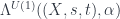
The older version of this paper talked about the untwisted version of the Dijkgraaf-Witten (DW for short) model, which is a certain kind of TQFT based on a gauge theory with a finite gauge group.  (Freed and Quinn put it as: “Chern-Simons theory with finite gauge group”).  The new version gets the general – that is, the twisted – form in the same way: factoring the theory into two parts. So, the DW model, which was originally described by Dijkgraaf and Witten in terms of a state-sum, is a functor

The “twisting” is the point of their paper, “Topological Gauge Theories and Group Cohomology”.  The twisting has to do with the action for some physical theory. Now, for a gauge theory involving flat connections, the kind of gauge-theory actions which involve the curvature of a connection make no sense: the curvature is zero.  So one wants an action which reflects purely global features of connections.  The cohomology of the gauge group is where this comes from.

Now, the machinery I describe is based on a point of view which has been described in a famous paper by Freed, Hopkins, Lurie and Teleman (FHLT for short – see further discussion here) in terms in which the two stages are called the “classical field theory” (which has values in groupoids), and the “quantization functor”, which takes one into Hilbert spaces.

Actually, we really want to have an “extended” TQFT: a TQFT gives a Hilbert space for each 2D manifold (“space”), and a linear map for a 3D cobordism (“spacetime”) between them. An extended TQFT will assign (higher) algebraic data to lower-dimension boundaries still.  My paper talks only about the case where we’ve extended down to codimension 2, whereas FHLT talk about extending “down to a point”. The point of this first stopping point is to unpack explicitly and computationally what the factorization into two parts looks like at the first level beyond the usual TQFT.

In the terminology I use, the classical field theory is:

This depends on a cohomology class . The “quantization functor” (which in this case I call “2-linearization”):

The middle stage involves the monoidal 2-category I call .  (In FHLT, they use different terminology, for instance “families” rather than “spans”, but the principle is the same.)

Freed and Quinn looked at the quantization of the “extended” DW model, and got a nice geometric picture. In it, the action is understood as a section of some particular line-bundle over a moduli space. This geometric picture is very elegant once you see how it works, which I found was a little easier in light of a factorization through .

This factorization isolates the geometry of this particular situation in the “classical field theory” – and reveals which of the features of their setup (the line bundle over a moduli space) are really part of some more universal construction.

In particular, this means laying out an explicit definition of both and .

2-Linearization Recalled

While I’ve talked about it before, it’s worth a brief recap of how 2-linearization works with a view to what happens when you twist it via groupoid cohomology. Here we have a 2-category , whose objects are groupoids (, , etc.), whose morphisms are spans of groupoids:

and whose 2-morphisms are spans of span-maps (taken up to isomorphism), which look like so:

(And, by the by: how annoying that WordPress doesn’t appear to support xypic figures…)

These form a (symmetric monoidal) 2-category, where composition of spans works by taking weak pullbacks.  Physically, the idea is that a groupoid has objects which are configurations (in the cause of gauge theory, connections on a manifold), and morphisms which are symmetries (gauge transformations, in this case).  Then a span is a groupoid of histories (connections on a cobordism, thought of as spacetime), and the maps pick out its starting and ending configuration.  That is, is the groupoid of flat -connections on a manifold , and is the groupoid of flat -connections on some cobordism , of which is part of the boundary.  So any such connection can be restricted to the boundary, and this restriction is .

Now 2-linearization is a 2-functor:

It gives a 2-vector space (a nice kind of category) for each groupoid .  Specifically, the category of its representations, .  Then a span turns into a functor which comes from “pulling” back along (the restricted representation where acts by first applying then the representation), then “pushing” forward along (to the induced representation).

What happens to the 2-morphisms is conceptually more complicated, but it depends on the fact that “pulling” and “pushing” are two-sided adjoints. Concretely, it ends up being described as a kind of “sum over histories” (where “histories” are the objects of ), which turns out to be exactly the path integral that occurs in the TQFT.

Or at least, it’s the path integral when the action is trivial! That is, if , so that what’s integrated over paths (“histories”) is just . So one question is: is there a way to factor things in this way if there’s a nontrivial action?

Cohomological Twisting

The answer is by twisting via cohomology. First, let’s remember what that means…

We’re talking about groupoid cohomology for some groupoid (which you can take to be a group, if you like).  “Cochains” will measure how much some nice algebraic fact, such as being a homomorphism, or being associative, “fails to occur”.  “Twisting by a cocycle” is a controlled way to force some such failure to happen.

So, an -cocycle is some function of composable morphisms of (or, if there’s only one object, “group elements”, which amounts to the same thing).  It takes values in some group of coefficients, which for us is always . 

The trivial case where is actually slightly subtle: a 0-cocycle is an invariant function on the objects of a groupoid. (That is, it takes the same value on any two objects related by an (iso)morphism. (Think of the object as a sequence of zero composable morphisms: it tells you where to start, but nothing else.)

The case is maybe a little more obvious. A 1-cochain  can measure how a function on objects might fail to be a 0-cocycle. It is a -valued function of morphisms (or, if you like, group elements).  The natural condition to ask for is that it be a homomorphism:

This condition means that a cochain is a cocycle. They form an abelian group, because functions satisfying the cocycle condition are closed under pointwise multiplication in . It will automatically by satisfied for a coboundary (i.e. if comes from a function on objects as ). But not every cocycle is a coboundary: the first cohomology is the quotient of cocycles by coboundaries. This pattern repeats.

It’s handy to think of this condition in terms of a triangle with edges , , and .  It says that if we go from the source to the target of the sequence with or without composing, and accumulate -values, our gives the same result.  Generally, a cocycle is a cochain satisfying a “coboundary” condition, which can be described in terms of an -simplex, like this triangle. What about a 2-cocycle? This describes how composition might fail to be respected.

So, for instance, a twisted representation of a group is not a representation in the strict sense. That would be a map into , such that .  That is, the group composition rule gets taken directly to the corresponding rule for composition of endomorphisms of the vector space .  A twisted representation only satisfies this up to a phase:

where is a function that captures the way this “representation” fails to respect composition.  Still, we want some nice properties: is a “cocycle” exactly when this twisting still makes respect the associative law:

Working out what this says in terms of , the cocycle condition says that for any composable triple we have:

So – the second group-cohomology group of – consists of exactly these which satisfy this condition, which ensures we have associativity.

Given one of these maps, we get a category of all the -twisted representations of . It behaves just like an ordinary representation category… because in fact it is one! It’s the category of representations of a twisted version of the group algebra of , called . The point is, we can use to twist the convolution product for functions on , and this is still an associative algebra just because satisfies the cocycle condition.

The pattern continues: a 3-cocycle captures how some function of 2 variable may fail to be associative: it specifies an associator map (a function of three variables), which has to satisfy some conditions for any four composable morphisms. A 4-cocycle captures how a map might fail to satisfy this condition, and so on. At each stage, the cocycle condition is automatically satisfied by coboundaries. Cohomology classes are elements of the quotient of cocycles by coboundaries.

So the idea of “twisted 2-linearization” is that we use this sort of data to change 2-linearization.

Twisted 2-Linearization

The idea behind the 2-category is that it contains , but that objects and morphisms also carry information about how to “twist” when applying the 2-linearization .  So in particular, what we have is a (symmetric monoidal) 2-category where:

• Objects consist of , where is a groupoid and $\theta \in Z^2(A,U(1))$
• Morphisms from to consist of a span from to , together with
• 2-Morphisms from to consist of a span from , together with

The cocycles have to satisfy some compatibility conditions (essentially, pullbacks of the cocycles from the source and target of a span should land in the same cohomology class).  One way to see the point of this requirement is to make twisted 2-linearization well-defined.

One can extend the monoidal structure and composition rules to objects with cocycles without too much trouble so that is a subcategory of . The 2-linearization functor extends to :

• On Objects: , the category of -twisted representation of
• On Morphisms: comes by pulling back a twisted representation in to one in , pulling it through the algebra map “multiplication by “, and pushing forward to
• On 2-Morphisms: For a span of span maps, one uses the usual formula (see the paper for details), but a sum over the objects picks up a weight of at each object

When the cocycles are trivial (evaluate to 1 always), we get back the 2-linearization we had before. Now the main point here is that the “sum over histories” that appears in the 2-morphisms now carries a weight.

So the twisted form of 2-linearization uses the same “pull-push” ideas as 2-linearization, but applied now to twisted representations. This twisting (at the object level) uses a 2-cocycle. At the morphism level, we have a “twist” between “pull” and “push” in constructing . What the “twist” actually means depends on which cohomology degree we’re in – in other words, whether it’s applied to objects, morphisms, or 2-morphisms.

The “twisting” by a 0-cocycle just means having a weight for each object – in other words, for each “history”, or connection on spacetime, in a big sum over histories. Physically, the 0-cocycle is playing the role of the Lagrangian functional for the DW model. Part of the point in the FHLT program can be expressed by saying that what Freed and Quinn are doing is showing how the other cocycles are also the Lagrangian – as it’s seen at higher codimension in the more “local” theory.

For a TQFT, the 1-cocycles associated to morphisms describe how to glue together values for the Lagrangian that are associated to histories that live on different parts of spacetime: the action isn’t just a number. It is a number only “locally”, and when we compose 2-morphisms, the 0-cocycle on the composite picks up a factor from the 1-morphism (or 0-morphism, for a horizontal composite) where they’re composed.

This has to do with the fact that connections on bits of spacetime can be glued by particular gauge transformations – that is, morphisms of the groupoid of connections. Just as the gauge transformations tell how to glue connections, the cocycles associated to them tell how to glue the actions. This is how the cohomological twisting captures the geometric insight that the action is a section of a line bundle – not just a function, which is a section of a trivial bundle – over the moduli space of histories.

So this explains how these cocycles can all be seen as parts of the Lagrangian when we quantize: they explain how to glue actions together before using them in a sum-over histories. Gluing them this way is essential to make sure that is actually a functor. But if we’re really going to see all the cocycles as aspects of “the action”, then what is the action really? Where do they come from, that they’re all slices of this bigger thing?

Twisting as Lagrangian

Now the DW model is a 3D theory, whose action is specified by a group-cohomology class . But this is the same thing as a class in the cohomology of the classifying space: . This takes a little unpacking, but certainly it’s helpful to understand that what cohomology classes actually classify are… gerbes. So another way to put a key idea of the FHLT paper, as Urs Schreiber put it to me a while ago, is that “the action is a gerbe on the classifying space for fields“.

What does this mean?

This map is given as a path integral over all connections on the space(-time) , which is actually just a sum, since the gauge group is finite and so all the connections are flat.  The point is that they’re described by assigning group elements to loops in :

But this amounts to the same thing as a map into the classifying space of :

This is essentially the definition of , and it implies various things, such as the fact that is a space whose fundamental group is , and has all other homotopy groups trivial. That is, is the Eilenberg-MacLane space . But the point is that the groupoid of connections and gauge transformations on just corresponds to the mapping space . So the groupoid cohomology classes we get amount to the same thing as cohomology classes on this space. If we’re given , then we can get at these by “transgression” – which is very nicely explained in a paper by Simon Willerton.

The essential idea is that a 3-cocycle (representing the class ) amounts to a nice 3-form on which we can integrate over a 3-dimentional submanifold to get a number. For a -dimensional , we get such a 3-manifold from a -dimensional submanifold of : each point gives a copy of in . Then we get a -cocycle on whose values come from integrating over this image. Here’s a picture I used to illustrate this in my talk:

Now, it turns out that this gives 2-cocycles for 1-manifolds (the objects of , 1-cocycles on 2D cobordisms between them, and 0-cocycles on 3D cobordisms between these cobordisms. The cocycles are for the groupoid of connections and gauge transformations in each case. In fact, because of Stokes’ theorem in , these have to satisfy all the conditions that make them into objects, morphisms, and 2-morphisms of . This is the geometric content of the Lagrangian: all the cocycles are really “reflections” of as seen by transgression: pulling back along the evaluation map from the picture. Then the way you use it in the quantization is described exactly by .

What I like about this is that is a fairly universal sort of thing – so while this example gets its cocycles from the nice geometry of which Freed and Quinn talk about, the insight that an action is a section of a (twisted) line bundle, that actions can be glued together in particular ways, and so on… These presumably can be moved to other contexts.

 

Benabou on Spans and Profunctors/Distributors

So I recently got back from a trip to the UK – most of the time was spent in Cardiff, at a workshop on TQFT and categorification at the University of Cardiff.  There were two days of talks, which had a fair amount of overlap with our workshop in Lisbon, so, being a little worn out on the topic, I’ll refrain from summarizing them all, except to mention a really nice one by Jeff Giansiracusa (who hadn’t been in Lisbon) which related (open/closed) TQFT’s and cohomology theories via a discussion of how categories of cobordisms with various kinds of structure correspond to various sorts of operads.  For example, the “little disks” operad, which describes the structure of how to compose disks with little holes, by pasting new disks into the holes of the old ones, corresponds to the usual cobordism category.

This workshop was part of a semester-long program they’ve been having, sponsored by an EU network on noncommutative geometry.  After the workshop was done, Tim Porter and I stayed on for the rest of the week to give some informal seminars and talk to the various grad students who were visiting at the time.  The seminars started off being directed by questions, but ended up talking about TQFT’s and their relations to various kinds of algebras and higher categorical structures, via classifying spaces.  We also had some interesting discussions outside these, for example with Jennifer Maier, who’s been working with Thomas Nicklaus on equivariant Dijkgraaf-Witten theory; with Grace Kennedy, about planar algebras and their relationships to TQFT‘s. I’d also like to give some credit to Makoto Yamashita, who’s interested in noncommutative geometry (viz) and pointed out to me a paper of Alain Connes which gives an account of integration on groupoids, and what corresponds to measures in that setting, which thankfully agrees with what little of it I’d been able to work out on my own.

---

However, what I’d like to take the time to write up was from the earlier part of my trip, where I visited with Jamie Vicary at Oxford. While I was there, I gave a little lunch seminar about the bicategory (actually a tricategory), and some of the physics- and TQFT-related uses for it. That turned out to be very apropos, because they also had another visitor at the same time, namely Jean Benabou, the fellow who invented bicategories, and introduced the idea of bicategories of spans as one of the first examples.  He gave a talk while I was there which was about the relationship between spans and what he calls “distributors” (which are often called “profunctors“, but since he was anyway the one who introduced them and gave them that name in the first place, and since he has since decided that “profunctors” should refer to only a special class of these entities, I’ll follow his terminology).

(Edit: Thanks to Thomas Streicher for passing on a reference to lecture notes he prepared from lecture by Benabou on the same general topic.)

The question to answer is: what is the relation between spans of categories and distributors?

This is related to a slightly lower-grade question about the relationship between spans of sets, and relations, although the answer turns out to be more complicated.  So, remember that a span from a set to a set is just a diagram like this: .  They can be composed together – so that given a span from to , and from to , we can take fibre products over and get a span from to , consisting of pairs of elements from the sets which map down to the same .  We can do the same thing in any category with pullbacks, not just .

A span is a relation if the pair of arrows is “jointly monic”, which is to say that as a map , it is a monomorphism – which, since we’re talking about sets, essentially means “a subset”.  That is, up to isomorphism of spans, just picks out a bunch of pairs , which are the “related” pairs in this relation.  So there is an inclusion .  What’s more  the inclusion has a left adjoin, which turns a span into a corresponding relation.  It follows from the fact that has an “epi-mono factorization”: namely, the map that comes from the span (and the definition of product) will factor through the image.  That is, it is the composite , where the first part is surjective, and the second part is injective.  Then the inclusion is a relation.  So we say the inclusion of into is a reflection.  (This is a slightly misleading term: there’s an adjoint to the inclusion, but it’s not an adjoint equivalence.  “Reflecting” twice may not get you back where you started, or anywhere isomorphic to it.)

(Edit: Actually, this is a bit wrong.  See the comments below.  What’s true is that the hom-categories of have reflective inclusions into the hom-categories of .  Here, we think of as a 2-category because it’s naturally enriched in posets.  Then these reflective inclusions of hom-categories can be used to build  a lax functor from to – but not an actual functor.)

So a slightly more general question is: if is a monoidal category, and is a  “reflective subcategory“, can we make into a monoidal category just by defining (the product in ) to be the reflection of the original product?   This is the one-object version of a question about bicategories.  Namely, say that is a bicategory, and is a sub-bicategory such that every pair of objects gives a reflective subcategory: has a reflection.  Then can we “pull” the composition of morphisms in back to ?

The answer is no: this just doesn’t work in general.  For spans of sets, and relations, it works: composing spans essentially “counts paths” which relate elements and , whereas composing relations only keeps track of whether or not there is a path.  However, composing spans which come from relations, and then squashing them back down to relations again, agrees with the composite in (the squashing just tells whether the set of paths from to by a sequence of relations is empty or not).  But in the case of and some reflective subcategory – among other possible examples – associativity and unit axioms will break, unless the reflections are specially tuned.  This isn’t to say that we can’t make a monoidal category (or a bicategory).  It just means that pulling back or along the reflection won’t work.  But there is a theorem that says we can always promote such an inclusion into one where this works.

So what’s an instance of all this?  A distributor (again, often called “profunctor”) from a category to is actually a functor .  Then there’s a bicategory , where for each objects there’s a category .  Distributors represent, in some sense, a categorification of relations. (This observation follows the periodic table of category theory, in which a 1-category is a category, a 0-category is a set, and a (-1)-category is a truth value.  There’s a 1-category of relations, with hom-sets , and each one is a map from into truth values, specifying whether a pair is related.)

The most elementary example of a distributor is the “hom-set” construction, where , which is indeed covariant in and contravariant in .  A way to see the general case in that obviously determines a functor from into presheaves on : , where is the category .

In fact, given a functor , we can define two different distributors:

with

and

with

(Remember, these are functors from the product into : so they are just taking hom-sets here in in one direction or the other.)  This much is a tautology: putting a value in in leaves a free variable, but the point is that can be interpreted as a category of “big objects of “.  This is since the Yoneda embedding embeds by taking each object to the presentable presheaf which assigns each object the set of morphisms into , so has “extended” objects of .

So distributors like are “generalized functors” into – and the idea is that this is in roughly the same way that “distributions” are to be seen as “generalized functions”, hence the name.  (Benabou now prefers to use the name “profunctor” to refer only to those distributors which map to “pro-objects” in , which are just special presheaves, namely the “flat” ones.)

Now we have an idea that there is a bicategory , whose hom-categories consist of distributors (and natural transformations), and that the usual functors (which can be seen as distributors which only happen to land in the image of under the Yoneda embedding) form a sub-bicategory: that is, post-composition with turns a functor into a distributor.

But moreover, this operation has an adjoint: functors out of can be “lifted” to functors out of , just by taking the Kan extension of a functor along .  This will work (pointwise, even), as long as is cocomplete, so that we can basically “add up” contributions from the objects of by taking colimits.  In the special case where for some other category , then this tells us how to get composition of distributors .

Now, for a functor , there are straightforward unit and counit natural transformations which makes (the image of under the embedding of into ) a left adjoint for .  So we’ve embedded into in such a way that every functor has a right adjoint.  What about ?  In general, given a bicategory , we can construe as a tricategory, which contains , in such a way that every morphism of has an ambidextrous adjoint (both left and right adjoint).  (There’s work on this by Toby Kenney and Dorette Pronk, and Alex Hoffnung has also been looking at this recently.)  So how does relate to ?

One statement is that a distributor can be seen as a special kind of span, namely:

where consists of all the “elements of ” (in particular, pasting together all the images in of pairs and the set maps that come from morphisms between them in ).  (As an aside: Benabou also explained how a cospan, can be got from a distributor.  The objects of are just the disjoint union of those from and , and the hom-sets are just taken from either , or , or as the sets given by , depending on the situation.  Then the span we just described completes a pullback square opposite this cospan – it’s a comma category.)

These spans end up having some special properties that result from how they’re constructed.  In particular, will be an op-fibration and will be a fibration (this, for instance, is alifting property that let one lift morphisms – since the morphisms are found as the images of the original distributor, this makes sense).  Also, the fibres of are discrete (these are by definition the images of identity morphisms, so naturally they’re discrete categories).  Finally, these properties (fibration, op-fibration, and discrete fibres) are enough to guarantee that a given span is (isomorphic to) one that comes from a distributor.  So we have an embedding .

What’s more, it’s a reflective embedding, because we can always mangle any span to get a new one where these properties hold: it’s enough to force fibres to be discrete by taking their – the connected components.  The other properties will then follow.  But notice that this is a very nontrivial thing to do: in general, the fibres of could be any sort of category, and this operation turns them into sets (of isomorphism classes).  So there’s an adjunction between and , and is a reflective sub-bicategory of .  But the severity of ends up meaning that this doesn’t get along well with composition – the composition of distributors (described above) is not related to composition of spans (which works by weak pullback) via this reflection in a naive way.  However, the theorem mentioned above means that there will be SOME reflecction that makes the compositions get along.  It just may not be as nice as this one.

This is kind of surprising, and the ideal punchline to go here would be to say what that reflection is like, but I don’t know the answer to that question just now.  Anyone else know?

---

Thanks to Bob Coecke, here are some pictures of me, a few of the people from ComLab, and Jean Benabou at dinner at the Oxford University Club, with a variety of dopey expressions as Bob snapped the pictures unexpectedly.  Thanks Bob.

 

Categorifying the Heisenberg Algebra

Marco Mackaay recently pointed me at a paper by Mikhail Khovanov, which describes a categorification of the Heisenberg algebra (or anyway its integral form ) in terms of a diagrammatic calculus.  This is very much in the spirit of the Khovanov-Lauda program of categorifying Lie algebras, quantum groups, and the like.  (There’s also another one by Sabin Cautis and Anthony Licata, following up on it, which I fully intend to read but haven’t done so yet. I may post about it later.)

Now, as alluded to in some of the slides I’ve from recent talks, Jamie Vicary and I have been looking at a slightly different way to answer this question, so before I talk about the Khovanov paper, I’ll say a tiny bit about why I was interested.

Groupoidification

The Weyl algebra (or the Heisenberg algebra – the difference being whether the commutation relations that define it give real or imaginary values) is interesting for physics-related reasons, being the algebra of operators associated to the quantum harmonic oscillator.  The particular approach to categorifying it that I’ve worked with goes back to something that I wrote up here, and as far as I know, originally was suggested by Baez and Dolan here.  This categorification is based on “stuff types” (Jim Dolan’s term, based on “structure types”, a.k.a. Joyal’s “species”).  It’s an example of the groupoidification program, the point of which is to categorify parts of linear algebra using the category .  This has objects which are groupoids, and morphisms which are spans of groupoids: pairs of maps .  Since I’ve already discussed the backgroup here before (e.g. here and to a lesser extent here), and the papers I just mentioned give plenty more detail (as does “Groupoidification Made Easy“, by Baez, Hoffnung and Walker), I’ll just mention that this is actually more naturally a 2-category (maps between spans are maps making everything commute).  It’s got a monoidal structure, is additive in a fairly natural way, has duals for morphisms (by reversing the orientation of spans), and more.  Jamie Vicary and I are both interested in the quantum harmonic oscillator – he did this paper a while ago describing how to construct one in a general symmetric dagger-monoidal category.  We’ve been interested in how the stuff type picture fits into that framework, and also in trying to examine it in more detail using 2-linearization (which I explain here).

Anyway, stuff types provide a possible categorification of the Weyl/Heisenberg algebra in terms of spans and groupoids.  They aren’t the only way to approach the question, though – Khovanov’s paper gives a different (though, unsurprisingly, related) point of view.  There are some nice aspects to the groupoidification approach: for one thing, it gives a nice set of pictures for the morphisms in its categorified algebra (they look like groupoids whose objects are Feynman diagrams).  Two great features of this Khovanov-Lauda program: the diagrammatic calculus gives a great visual representation of the 2-morphisms; and by dealing with generators and relations directly, it describes, in some sense¹, the universal answer to the question “What is a categorification of the algebra with these generators and relations”.  Here’s how it works…

Heisenberg Algebra

One way to represent the Weyl/Heisenberg algebra (the two terms refer to different presentations of isomorphic algebras) uses a polynomial algebra .  In fact, there’s a version of this algebra for each natural number (the stuff-type references above only treat , though extending it to “-sorted stuff types” isn’t particularly hard).  In particular, it’s the algebra of operators on generated by the “raising” operators and the “lowering” operators .  The point is that this is characterized by some commutation relations.  For , we have:

but on the other hand

So the algebra could be seen as just a free thing generated by symbols with these relations.  These can be understood to be the “raising and lowering” operators for an -dimensional harmonic oscillator.  This isn’t the only presentation of this algebra.  There’s another one where (as in ) has a slightly different interpretation, where the and operators are the position and momentum operators for the same system.  Finally, a third one – which is the one that Khovanov actually categorifies – is skewed a bit, in that it replaces the with a different set of so that the commutation relation actually looks like

It’s not instantly obvious that this produces the same result – but the can be rewritten in terms of the , and they generate the same algebra.  (Note that for the one-dimensional version, these are in any case the same, taking .)

Diagrammatic Calculus

To categorify this, in Khovanov’s sense (though see note below¹), means to find a category whose isomorphism classes of objects correspond to (integer-) linear combinations of products of the generators of .  Now, in the setup, we can say that the groupoid , or equvialently , represents Fock space.  Groupoidification turns this into the free vector space on the set of isomorphism classes of objects.  This has some extra structure which we don’t need right now, so it makes the most sense to describe it as , the space of power series (where corresponds to the object ).  The algebra itself is an algebra of endomorphisms of this space.  It’s this algebra Khovanov is looking at, so the monoidal category in question could really be considered a bicategory with one object, where the monoidal product comes from composition, and the object stands in formally for the space it acts on.  But this space doesn’t enter into the description, so we’ll just think of as a monoidal category.  We’ll build it in two steps: the first is to define a category .

The objects of are defined by two generators, called and , and the fact that it’s monoidal (these objects will be the categorifications of and ).  Thus, there are objects and so forth.  In general, if is some word on the alphabet , there’s an object .

As in other categorifications in the Khovanov-Lauda vein, we define the morphisms of to be linear combinations of certain planar diagrams, modulo some local relations.  (This type of formalism comes out of knot theory – see e.g. this intro by Louis Kauffman).  In particular, we draw the objects as sequences of dots labelled or , and connect two such sequences by a bunch of oriented strands (embeddings of the interval, or circle, in the plane).  Each dot is the endpoint of a strand oriented up, and each dot is the endpoint of a strand oriented down.  The local relations mean that we can take these diagrams up to isotopy (moving the strands around), as well as various other relations that define changes you can make to a diagram and still represent the same morphism.  These relations include things like:

which seems visually obvious (imagine tugging hard on the ends on the left hand side to straighten the strands), and the less-obvious:

and a bunch of others.  The main ingredients are cups, caps, and crossings, with various orientations.  Other diagrams can be made by pasting these together.  The point, then, is that any morphism is some -linear combination of these.  (I prefer to assume most of the time, since I’m interested in quantum mechanics, but this isn’t strictly necessary.)

The second diagram, by the way, are an important part of categorifying the commutation relations.  This would say that (the commutation relation has become a decomposition of a certain tensor product).  The point is that the left hand sides show the composition of two crossings and in two different orders.  One can use this, plus isotopy, to show the decomposition.

That diagrams are invariant under isotopy means, among other things, that the yanking rule holds:

(and similar rules for up-oriented strands, and zig zags on the other side).  These conditions amount to saying that the functors and are two-sided adjoints.  The two cups and caps (with each possible orientation) give the units and counits for the two adjunctions.  So, for instance, in the zig-zag diagram above, there’s a cup which gives a unit map (reading upward), all tensored on the right by .  This is followed by a cap giving a counit map (all tensored on the left by ).  So the yanking rule essentially just gives one of the identities required for an adjunction.  There are four of them, so in fact there are two adjunctions: one where is the left adjoint, and one where it’s the right adjoint.

Karoubi Envelope

Now, so far this has explained where a category comes from – the one with the objects described above.  This isn’t quite enough to get a categorification of : it would be enough to get the version with just one and one element, and their powers, but not all the and .  To get all the elements of the (integral form of) the Heisenberg algebras, and in particular to get generators that satisfy the right commutation relations, we need to introduce some new objects.  There’s a convenient way to do this, though, which is to take the Karoubi envelope of .

The Karoubi envelope of any category is a universal way to find a category that contains and for which all idempotents split (i.e. have corresponding subobjects).  Think of vector spaces, for example: a map such that is a projection.  That projection corresponds to a subspace , and is actually another object in , so that splits (factors) as .  This might not happen in any general , but it will in .  This has, for objects, all the pairs where is idempotent (so is contained in as the cases where ).  The morphisms are just maps with the compatibility condition that (essentially, maps between the new subobjects).

So which new subobjects are the relevant ones?  They’ll be subobjects of tensor powers of our .  First, consider .  Obviously, there’s an action of the symmetric group on this, so in fact (since we want a -linear category), its endomorphisms contain a copy of , the corresponding group algebra.  This has a number of different projections, but the relevant ones here are the symmetrizer,:

which wants to be a “projection onto the symmetric subspace” and the antisymmetrizer:

which wants to be a “projection onto the antisymmetric subspace” (if it were in a category with the right sub-objects). The diagrammatic way to depict this is with horizontal bars: so the new object (the symmetrized subobject of ) is a hollow rectangle, labelled by .  The projection from is drawn with arrows heading into that box:

The antisymmetrized subobject is drawn with a black box instead.  There are also and defined in the same way (and drawn with downward-pointing arrows).

The basic fact – which can be shown by various diagram manipulations, is that .  The key thing is that there are maps from the left hand side into each of the terms on the right, and the sum can be shown to be an isomorphism using all the previous relations.  The map into the second term involves a cap that uses up one of the strands from each term on the left.

There are other idempotents as well – for every partition of , there’s a notion of -symmetric things – but ultimately these boil down to symmetrizing the various parts of the partition.  The main point is that we now have objects in corresponding to all the elements of .  The right choice is that the   (the new generators in this presentation that came from the lowering operators) correspond to the (symmetrized products of “lowering” strands), and the correspond to the (antisymmetrized products of “raising” strands).  We also have isomorphisms (i.e. diagrams that are invertible, using the local moves we’re allowed) for all the relations.  This is a categorification of .

Some Generalities

This diagrammatic calculus is universal enough to be applied to all sorts of settings where there are functors which are two-sided adjoints of one another (by labelling strands with functors, and the regions of the plane with categories they go between).  I like this a lot, since biadjointness of certain functors is essential to the 2-linearization functor (see my link above).  In particular, uses biadjointness of restriction and induction functors between representation categories of groupoids associated to a groupoid homomorphism (and uses these unit and counit maps to deal with 2-morphisms).  That example comes from the fact that a (finite-dimensional) representation of a finite group(oid) is a functor into , and a group(oid) homomorphism is also just a functor .  Given such an , there’s an easy “restriction” , that just works by composing with .  Then in principle there might be two different adjoints , given by the left and right Kan extension along .  But these are defined by colimits and limits, which are the same for (finite-dimensional) vector spaces.  So in fact the adjoint is two-sided.

Khovanov’s paper describes and uses exactly this example of biadjointness in a very nice way, albeit in the classical case where we’re just talking about inclusions of finite groups.  That is, given a subgroup , we get a functors , which just considers the obvious action of act on any representation space of .  It has a biadjoint , which takes a representation of to , which is a special case of the formula for a Kan extension.  (This formula suggests why it’s also natural to see these as functors between module categories and ).  To talk about the Heisenberg algebra in particular, Khovanov considers these functors for all the symmetric group inclusions .

Except for having to break apart the symmetric groupoid as , this is all you need to categorify the Heisenberg algebra.  In the categorification, we pick out the interesting operators as those generated by the map from to itself, but “really” (i.e. up to equivalence) this is just all the inclusions taken at once.  However, Khovanov’s approach is nice, because it separates out a lot of what’s going on abstractly and uses a general diagrammatic way to depict all these 2-morphisms (this is explained in the first few pages of Aaron Lauda’s paper on ambidextrous adjoints, too).  The case of restriction and induction is just one example where this calculus applies.

There’s a fair bit more in the paper, but this is probably sufficient to say here.

---

¹ There are two distinct but related senses of “categorification” of an algebra here, by the way.  To simplify the point, say we’re talking about a ring .  The first sense of a categorification of is a (monoidal, additive) category with a “valuation” in that takes to and to .  This is described, with plenty of examples, in this paper by Rafael Diaz and Eddy Pariguan.  The other, typical of the Khovanov program, says it is a (monoidal, additive) category whose Grothendieck ring is .  Of course, the second definition implies the first, but not conversely.  The objects of the Grothendieck ring are isomorphism classes in .  A valuation may identify objects which aren’t isomorphic (or, as in groupoidification, morphisms which aren’t 2-isomorphic).

So a categorification of the first sort could be factored into two steps: first take the Grothendieck ring, then take a quotient to further identify things with the same valuation.  If we’re lucky, there’s a commutative square here: we could first take the category , find some surjection , and then find that .  This seems to be the relation between Khovanov’s categorification of and the one in . This is the sense in which it seems to be the “universal” answer to the problem.

 

Some different ideas of “state”, part 2: ensembles, 2-states, and selection sectors

I just posted the slides for “Groupoidification and 2-Linearization”, the colloquium talk I gave at Dalhousie when I was up in Halifax last week. I also gave a seminar talk in which I described the quantum harmonic oscillator and extended TQFT as examples of these processes, which covered similar stuff to the examples in a talk I gave at Ottawa, as well as some more categorical details.

Now, in the previous post, I was talking about different notions of the “state” of a system – all of which are in some sense “dual to observables”, although exactly what sense depends on which notion you’re looking at. Each concept has its own particular “type” of thing which represents a state: an element-of-a-set, a function-on-a-set, a vector-in-(projective)-Hilbert-space, and a functional-on-operators. In light of the above slides, I wanted to continue with this little bestiary of ontologies for “states” and mention the versions suggested by groupoidification.

State as Generalized Stuff Type

This is what groupoidification introduces: the idea of a state in . As I said in the previous post, the key concepts behind this program are state, symmetry, and history. “State” is in some sense a logical primitive here – given a bunch of “pure” states for a system (in the harmonic oscillator, you use the nonnegative integers, representing n-photon energy states of the oscillator), and their local symmetries (the -particle state is acted on by the permutation group on elements), one defines a groupoid.

So at a first approximation, this is like the “element of a set” picture of state, except that I’m now taking a groupoid instead of a set. In a more general language, we might prefer to say we’re talking about a stack, which we can think of as a groupoid up to some kind of equivalence, specifically Morita equivalence. But in any case, the image is still that a state is an object in the groupoid, or point in the stack which is just generalizing an element of a set or point in configuration space.

However, what is an “element” of a set ? It’s a map into from the terminal element in , which is “the” one-element set – or, likewise, in , from the terminal groupoid, which has only one object and its identity morphism. However, this is a category where the arrows are set maps. When we introduce the idea of a “history “, we’re moving into a category where the arrows are spans, (which by abuse of notation sometimes gets called but more formally ). A span represents a set/groupoid/stack of histories, with source and target maps into the sets/groupoids/stacks of states of the system at the beginning and end of the process represented by .

Then we don’t have a terminal object anymore, but the same object is still around – only the morphisms in and out are different. Its new special property is that it’s a monoidal unit. So now a map from the monoidal unit is a span . Since the map on the left is unique, by definition of “terminal”, this really just given by the functor , the target map. This is a fibration over , called here for “phi”-bration, but this is appropriate, since it corresponds to what’s usually thought of as a wavefunction .

This correspondence is what groupoidification is all about – it has to do with taking the groupoid cardinality of fibres, where a “phi”bre of is the essential preimage of an object – everything whose image is isomorphic to . This gives an equivariant function on – really a function of isomorphism classes. (If we were being crude about the symmetries, it would be a function on the quotient space – which is often what you see in real mechanics, when configuration spaces are given by quotients by the action of some symmetry group).

In the case where is the groupoid of finite sets and bijections (sometimes called ), these fibrations are the “stuff types” of Baez and Dolan. This is a groupoid with something of a notion of “underlying set” – although a forgetful functor (giving “underlying sets” for objects in a category ) is really supposed to be faithful (so that -morphisms are determined by their underlying set map). In a fibration, we don’t necessarily have this. The special case corresponds to “structure types” (or combinatorial species), where is a groupoid of “structured sets”, with an underlying set functor (actually, species are usually described in terms of the reverse, fibre-selecting functor , where the image of a finite set consists of the set of all “$\Phi$-structured” sets (such as: “graphs on set “, or “trees on “, etc.) The fibres of a stuff type are sets equipped with “stuff”, which may have its own nontrivial morphisms (for example, we could have the groupoid of pairs of sets, and the “underlying” functor selects the first one).

Over a general groupoid, we have a similar picture, but instead of having an underlying finite set, we just have an “underlying -object”. These generalized stuff types are “states” for a system with a configuration groupoid, in . Notice that the notion of “state” here really depends on what the arrows in the category of states are – histories (i.e. spans), or just plain maps.

Intuitively, such a state is some kind of “ensemble”, in statistical or quantum jargon. It says the state of affairs is some jumble of many configurations (which we apparently should see as histories starting from the vacuous unit ), each of which has some “underlying” pure state (such as energy level, or what-have-you). The cardinality operation turns this into a linear combination of pure states by defining weights for each configuration in the ensemble collected in .

2-State as Representation

A linear combination of pure states is, as I said, an equivariant function on the objects of . It’s one way to “categorify” the view of a state as a vector in a Hilbert space, or map from (i.e. a point in the projective Hilbert space of lines in the Hilbert space ), which is really what’s defined by one of these ensembles.

The idea of 2-linearization is to categorify, not a specific state , but the concept of state. So it should be a 2-vector in a 2-Hilbert space associated to . The Hilbert space was some space of functions into $mathbb{C}$, which we categorify by taking instead of a base field, a base category, namely . A 2-Hilbert space will be a category of functors into – that is, the representation category of the groupoid .

(This is all fine for finite groupoids. In the inifinte case, there are some issues: it seems we really should be thinking of the 2-Hilbert space as category of representations of an algebra. In the finite case, the groupoid algebra is a finite dimensional C*-algebra – that is, just a direct sum (over iso. classes of objects) of matrix algebras, which are the group algebras for the automorphism groups at each object. In the infinite dimensional world, you probable should be looking at the representations of the von Neumann algebra completion of the C*-algebra you get from the groupoid. There are all sorts of analysis issues about measurability that lurk in this area, but they don’t really affect how you interpret “state” in this picture, so I’ll skip it.)

A “2-state”, or 2-vector in this Hilbert space, is a representation of the groupoid(-algebra) associated to the system. The “pure” states are irreducible representations – these generate all the others under the operations of the 2-Hilbert space (“sum”, “scalar product”, etc. in their 2-vector space forms). Now, an irreducible representation of a von Neumann algebra is called a “superselection sector” for a quantum system. It’s playing the role of a pure state here.

There’s an interesting connection here to the concept of state as a functional on a von Neumann algebra. As I described in the last post, the GNS representation associates a representation of the algebra to a state. In fact, the GNS representation is irreducible just when the state is a pure state. But this notion of a superselection sector makes it seem that the concept of 2-state has a place in its own right, not just by this correspondence.

So: if a quantum system is represented by an algebra of operators on a Hilbert space , that representation is a direct sum (or direct integral, as the case may be) of irreducible ones, which are “sectors” of the theory, in that any operator in can’t take a vector out of one of these “sectors”. Physicists often associate them with conserved quantities – though “superselection” sectors are a bit more thorough: a mere “selection sector” is a subspace where the projection onto it commutes with some subalgebra of observables which represent conserved quantities. A superselection sector can equivalently be defined as a subspace whose corresponding projection operator commutes with EVERYTHING in . In this case, it’s because we shouldn’t have thought of the representation as a single Hilbert space: it’s a 2-vector in – but as a direct integral of some Hilbert bundle that lives on the space of irreps. Those projections are just part of the definition of such a bundle. The fact that acts on this bundle fibre-wise is just a consequence of the fact that the total is a space of sections of the “2-state”. These correspond to “states” in usual sense in the physical interpretation.

Now, there are 2-linear maps that intermix these superselection sectors: the ETQFT picture gives nice examples. Such a map, for example, comes up when you think of two particles colliding (drawn in that world as the collision of two circles to form one circle). The superselection sectors for the particles are labelled by (in one special case) mass and spin – anyway, some conserved quantities. But these are, so to say, “rest mass” – so there are many possible outcomes of a collision, depending on the relative motion of the particles. So these 2-maps describe changes in the system (such as two particles becoming one) – but in a particular 2-Hilbert space, say for some groupoid describing the current system (or its algebra), a 2-state is a representation of the of the resulting system). A 2-state-vector is a particular representation. The algebra can naturally be seen as a subalgebra of the automorphisms of .

So anyway, without trying to package up the whole picture – here are two categorified takes on the notion of state, from two different points of view.

I haven’t, here, got to the business about Tomita flows coming from states in the von Neumann algebra sense: maybe that’s to come.

 

Paper: Double Bicategories and Double Cospans

So this paper of mine was recently accepted by the Journal of Homotopy and Related Structures (the version that was accepted should be reflected on the arXiv by tomorrow – i.e. July 10 – I’m not sure about the journal ). It’s been a while since I sent out the earliest version, and most of the changes have involved figuring out who the audience is, and consequently what could be left out. I guess that’s a side-effect of taking an excerpt from my thesis, which was much longer. In any case, it now seems to have reached a final point. Some of what was in it – the section about cobordisms – is now in a paper (in progress) about TQFT. I don’t see anywhere else to include the other missing bit, however, which has to do with Lawvere theories, and since I just wrote a bunch about MakkaiFest, I thought I might include some of that here.

The paper came about because I was trying to write my thesis, which describes an extended TQFT as a 2-functor (and considers how it could produce a version of 3D quantum gravity). The 2-functor

(or into ) is an ETQFT. The construction of the 2-functor uses the fact that you can get spans of groupoids out of cospans of manifolds – and in particular, out of cobordisms. One problem is how to describe so that this works. It’s actually most naturally a cubical 2-category of some kind. The strict version of this concept is a double category – which has (in principle separate) categories of horizontal and vertical of morphisms, as well as square 2-cells. Ideally, one would like a “weak” version, where composition of squares and morphisms can be only weakly associative (and have weak unit laws). A “pseudocategory” implements this where the only higher-dimensional morphisms are the squares, but it turns out to be strict in one direction, and weak in the other. As it happens, it’s a big pain to use only squares for the 2-morphisms.

Initially it seemed I would have to define a whole new structure to get weak composition in both directions, because in both directions, composition represents gluing bits of manifolds together along boundaries – using a diffeomorphism (or a smooth homeomorphism, depending on which kind of manifolds we’re dealing with). I called it a “double bicategory” and started trying to define it along the same lines as a double category. It then turned out that Dominic Verity had already defined a “double bicategory” – you can read the paper where I talk about how the notions are related. Here I want to talk about a few aspects which I cut out of the paper along the way.

The idea is that there are two ways of “categorifying”: internalization, and enrichment. A bicategory is a category enriched in , the category of categories – for any two elements, there’s a whole hom-category of morphisms (and 2-morphisms). A double category is a category internal to . This means you can think of it as a category of objects and a category of morphisms, equipped with functors satisfying all the usual properties for the maps in the definition of a category: composition functors, unit functors, and so forth. This definition turns out to be equivalent to the usual one. So I thought: why not do the same with bicategories?

Thus, the way I defined double bicategory was: “A bicategory internal to “. In the paper as it stands, that’s all I say. What I cut out was a sort of dangling loose end pointing toward Lawvere theories – or rather, a variant thereof – finite limit theories (for something more detailed, see this recent paper by Lack and Rosicky). As I mentioned in the previous post, a Lawvere theory is an approach to universal algebra – it formally defines a kind of object (e.g. group, ring, abelian group, etc.) as a functor from a category which is the “theory” of such objects, while the functor is a “model” of the theory.

What makes it “universal” algebra is that it can involve definitions with many sorts of objects, many operations, given as arrows, of different arities (number of inputs and outputs). This last makes sense in the monoidal context, and in particular Cartesian. Making decisions like this – what class of categories and functors we’re dealing with – specifies which doctrine the theory lives in. In the case of bicategories, this is the doctrine of categories with finite limits. In a Lawvere theory in the original sense, the doctrine is categories with finite products – so if there’s an object , there are also objects for all . Then there are things like multiplication maps and so on. For a category or bicategory, multiplication might be partial – so we need finite limits. A model of a theory in this doctrine is a limit-preserving functor.

So what does the theory of bicategories look like? It’s easy enough to see if you think that a (small) bicategory is a “bicategory in “, and reproduce the usual definition, omitting reference to sets. It has objects , , and . (This fact already means this is a “multi-sorted” theory, which goes beyond what can be done with another approach to universal algebra based on monads). Funthermore, there are maps between these objects, interpreted as source, target, and identity maps of various sorts. These form diagrams, and since we’re in a finite limit theory, there must be various objects like which for sets would have the interpretation “pairs of composable morphisms”. Then there’s a composition map … and so on. In short, in describing the axioms for a bicategory in a “nice” way (i.e. in terms of arrows, commuting diagrams, etc.), we’re giving a presentation of a certain category, , in generators and relations. Then a model of the theory is a functor – picking out a “bicategory in “.

Now, a bicategory in is a bicategory. But a bicategory in is another matter. First of all, I should say there’s something kind of odd here, since is most naturally regarded as a tricategory. However, we can regard it as a category by disregarding higher morphisms and taking 2-functors only up to equivalence to make into an honest category with associative composition. Thus, if we have a functor , we have:

• Bicategories , latex $F(Mor)$, and
• 2-Functors , and so on
• satisfying conditions implied by the bicategory axioms

But each of those bicategories (in !) has sets of objects, morphisms, and 2-morphisms, and one can break all the functors apart into three collections of maps acting on each of these three levels. They’ll satisfy all the conditions from the axioms – in fact, they make three new bicategories. So, for example, the object-sets of the bicategories , and form a bicategory using the object maps of the 2-functors and so on.

So if we say the original bicategories and so on are “horizontal”, and these new ones are “vertical”, we have something resembling a double category, but weak (since bicategories are weak) in both directions. The result is most naturally a four-dimensional structure (the 2-morphisms in are most conveniently drawn as 4d, which is shown in Table 2 of the paper).

Now, the paper as it is describes all this structure without explicitly mentioning the theory except in passing – one can define “internal bicategory” without it. This is why this is a “loose end” of this paper: a major benefit of using Lawvere-style theories is the availability of morphisms of theories, which don’t come up here.

In any case, with this 4D structure in hand, what I do in the paper is (a) get some conditions that allow one to decategorify it down to Verity’s version of “double bicategory” (and even down to a bicategory); and (b) show that couble cospans are an example (double spans would do equally well, but the application is to cobordisms, which are cospans). My own reason for wanting to get down to a 2D structure is the application to extended TQFT, which means we want a 2-category of cobordisms, thought of in terms of (co)spans.

Maybe in a subsequent post I’ll talk about the example itself, but one point about internalization does occur to me. Double cospans give an example of a double bicategory in the sense above – a strict model of in . In fact, they consist of “(co)spans of (co)spans” in a way that Marco Grandis formalized in terms of powers , where is the diagram (i.e. category) . One can actually think of this in terms of internalization: these are spans in a category whose objects are spans in , and whose morphisms are triples of maps in linking two spans (likewise for the span-map 2-morphisms). Yet it’s manifestly edge-symmetric: both the horizontal and vertical bicategories are the same.

As I mentioned in the previous post, there are lots of nice examples of double categories which are not edge-symmetric – sets, functions, and relations; or rings, homomorphisms, and bimodules, say. In fact, the second is only a pseudocategory – weak in one direction (composition of bimodules by tensor product is really only defined up to isomorphism). This is a significant thing about non-edge-symmetric examples. There’s much less motive for assuming both directions are equally strict. It’s also more natural in some ways: a pseudocategory is a weak model of in – equations in the theory are represented by (coherent) isomorphisms. This is the most general situation, and a strict model is a special case.

In the bicategory world, as I said, is a tricategory, so weaker models than the one I’ve given are possible – though they’re not symmetric, and so while one direction has composition and units as weak as a bicategory, the other direction will be weaker still. Robert Paré, in a conversation at MakkaiFest, suggested that a nice definition for a cubical n-category might have each direction being one step weaker than the previous one – a natural generalization of pseudocategories. Maybe there’s a way to make this seem natural in terms of internalization? One can iterate internalizing: having defined double bicategories, collect them together and find models of in , and so forth. Maybe doing this as weakly as possible would give this tower of increasing weakness.

Now, I don’t have a great punchline to sum all this up, except that internalization seems to be an interesting lens with which to look at cubical n-categories.

 

My Talk at “Categories, Quanta, Concepts”

I spent most of last week attending four of the five days of the workshop “Categories, Quanta, Concepts”, at the Perimeter Institute.  In the next few days I plan to write up many of the talks, but it was quite a lot.  For the moment, I’d like to do a little writeup on the talk I gave.  I wasn’t originally expecting to speak, but the organizers wanted the grad students and postdocs who weren’t talking in the scheduled sessions to give little talks.  So I gave a short version of this one which I gave in Ottawa but as a blackboard talk, so I have no slides for it.

Now, the workshop had about ten people from Oxford’s Comlab visiting, including Samson Abramsky and Bob Coecke, Marni Sheppard, Jamie Vicary, and about half a dozen others.  Many folks in this group work in the context of dagger compact categories, which is a nice abstract setting that captures a lot of the features of the category which are relevant to quantum mechanics.  Jamie Vicary had, earlier that day, given a talk about n-dimensional TQFT’s and n-categories – specifically, n-Hilbert spaces.  I’ll write up their talks in a later,  but it was a nice context in which to give the talk.

The point of this talk is to describe, briefly, – as a category and as a 2-category; to explain why it’s a good conceptual setting for quantum theory; and to show how it bridges the gap between Hilbert spaces and 2-Hilbert spaces.

History and Symmetry

In the course of an afternoon discussion session, we were talking about the various approaches people are taking in fundamentals of quantum theory, and in trying to find a “quantum theory of gravity” (whatever that ends up meaning).  I raised a question about robust ideas: basically, it seems to me that if an idea shows up across many different domains, that’s probably a sign it belongs in a good theory.  I was hoping people knew of a number of these notions, because there are really only two I’ve seen in this light, and really there probably should be more.

The two physical  notions that motivate everything here are (1) symmetry, and (2) emphasis on histories.  Both ideas are applied to states: states have symmetries; histories link starting states to ending states.  Combining them suggests histories should have symmetries of their own, which ought to get along with the symmetries of the states they begin and end with.

Both concepts are rather fundamental. Hermann Weyl wrote a whole book, “Symmetry”, about the first, and wrote: As far as I can see, all a-priori statements in physics are based on symmetry. From diffeomorphism invariance in general relativity, to gauge symmetry in quantum field theory, to symmetric tensor products involved in Fock space, through classical examples like Noether’s theorem. Noether’s theorem is also about histories: it applies when a symmetry holds along an entire history of a system: in fact, Langrangian mechanics generally is all about histories, and how they’re selected to be “real” in a classical system (by having a critical value of the action functional). The Lagrangian point of view appears in quantum theory (and this was what Richard Feynman did in his thesis) as the famous “sum over histories”, or path integral. General relativity embraces histories as real – they’re spacetimes, which is what GR is all about. So these concepts seem to hold up rather well across different contexts.

I began by drawing this table:

The names are all those of categories. Moving left to right moves from a category describing collections of states, to one describing states-and-histories. It so happens that it also takes a cartesian category (or 2-category) to a symmetric monoidal one. Moving from top to bottom goes from a setting with no symmetry to one with symmetry. In both cases, the key concept is naturally expressed with a category, and shows up in morphisms. Now, since groupoids are already categories, both of the bottom entries properly ought to be 2-categories, but when we choose to, we can ignore that fact.

Why Spans?

I’ve written a bunch on spans here before, but to recap, a span in a category is a diagram like: . Say we’re in , so all these objects are sets: we interpret and as sets of states. Each one describes some system by collecting all its possible (“pure”) states. (To be better, we could start with a different base category – symplectic manifolds, say – and see if the rest of the analysis goes through). For now, we just realize that is a set of histories leading the system to the system (notice there’s no assumption the system is the same). The maps are source and target maps: they specify the unique state where a history starts and where it ends.

If has pullbacks (or at least any we may need), we can use them to compose spans:

The pullback – a fibred product if we’re in – picks out pairs of histories in which match at . This should be exactly the possible histories taking to .

I’ve included an arrow to the category : this is the category whose objects are sets, and whose morphisms are relations. A number of people at CQC mentioned as an example of a monoidal category which supports toy models having some but not all features of quantum mechanics. It happens to be a quotient of . A relation is an equivalence class of spans, where we only notice whether the set of histories connecting to is empty or not. is more like quantum mechanics, because its composition is just like matrix multiplication: counting the number of histories from to turns the span into a matrix – so we can think of and as being like vector spaces.

In fact, there’s a map taking an object to and a span to the matrix I just mentioned, which faithfully represents . A more conceptual way to say this is: a function can be transported across the span. It lifts to as . Getting down the other leg, we add all the contributions of each history ending at a given : .

This “sum over histories” is what matrix multiplication actually is.

Why Groupoids?

The point of groupoids is that they represent sets with a notion of (local) symmetry. A groupoid is a category with invertible morphisms. Each such isomorphism tells us that two states are in some sense “the same”. The beginning example is the “action groupoid” that comes from a group acting on a set , which we call (or the “weak quotient” of by ).

This suggests how groupoids come into the physical picture – the intuition is that is the set (or, in later variations, space) of states, and is a group of symmetries.  For example, could be a group of coordinate transformations: states which can be transformed into each other by a rotation, say, are formally but not physically different.  The Extended TQFT example comes from the case where is a set of connections, and the group of gauge transformations.  Of course, not all physically interesting cases come from a single group action: for the harmonic oscillator, the states (“pure states”) are just energy levels – nonnegative integers.  On each state , there is an action of the permutation group – a “local” symmetry.

One nice thing about groupoids is that one often really only wants to think about them up to equivalence – as a result, it becomes a matter of convention whether formally different but physically indistinguishable states are really considered different.  There’s a side effect, though: is a 2-category.  In particular, this has two consequences for : it ought to have 2-morphisms, so we stop thinking about spans up to isomorphism.  Instead, we allow spans of span maps as 2-morphisms.  Also, when composing spans (which are no longer taken up to isomorphism) we have to use a weak pullback, not an ordinary one.  I didn’t have time to say much about the 2-morphism level in the CQC talk, but the slides above do.

In any case, moving into means that the arrows in the spans are now functors – in particular, a symmetry of a history  now has to map to a symmetry of the start and end states, and .  In particular, the functors give homomorphisms of the symmetry groups of each object.

Physics in Hilb and 2Hilb

So the point of the above is really to motivate the claim that there’s a clear physical meaning to groupoids (states and symmetries), and spans of them (putting histories on an even footing with states).  There’s less obvious physical meaning to the usual setting of quantum theory, the category – but it’s a slightly nicer category than .  For one thing, there is a concept of a “dual” of a span – it’s the same span, with the roles of and interchanged.  However (as Jamie Vicary pointed out to me), it’s not an “adjoint” in in the technical sense.  In particular, is a symmetric monoidal category, like , but it’s not “dagger compact”, the kind of category all the folks from Oxford like so much.

Now, groupoidification lets us generalize the map to groupoids making as few changes as possible.  We still use Hilbert space , but now is the set of isomorphism classes of objects in the groupoid.  The “sum over histories” – in other words, the linear map associated to a span – is found in almost the same way, but histories now have “weights” found using groupoid cardinality (see any of the papers on groupoidification, or my slides above, for the details).  This reproduces a lot of known physics (see my paper on the harmonic oscillator; TQFT’s can also be defined this way).

While this is “as much like” linearization of as possible in some sense, it’s not exactly analogous.  It also is rather violent to the structure of the groupoids: at the level of objects it treats as . At the morphism level, it ignores everything about the structure of symmetries in the system except how many of them there are.   Since a groupoid is a category, the more direct analogy for – the set of functions (fancier versions use, say, functions only) from to is – the category of functors from a groupoid into .  That is, representations of .

One of the attractions here is that, because of a generalization of Tanaka-Krein duality, this category will actually be enough to reconstruct the groupoid if it’s reasonably nice.  The representation of in , unlike in is actually faithful for objects, at least for compact or finite groupoids.

Then you can “pull and push” a representation across a span to get – using , the adjoint functor to pulling back.  This is the 1-morphism level of the 2-functor I call , generalizing the functor in the world of sets.  The result is still a “direct sum over histories” – but because we’re dealing with pushing representations through homomorphisms, this adjoint is a bit more complicated than in the 0-category world of .  (See my slides or paper for the details).  But it remains true that the weights and so forth used in ordinary groupoidification show up here at the level of 2-morphisms.  So the representation in is not a faithful representation of the (intuitively meaningful) category either.  But it does capture a fair bit more than Hilbert spaces.

One point of my talk was to try to motivate the use of 2-Hilbert spaces in physics from an a-priori point of view.  One thing I think is nice, for this purpose, is to see how our physical intuitions motivate – a nice point itself – and then observe that there is this “higher level” span around:

Further Thoughts

Where can one take this?  There seem to be theories whose states and symmetries naturally want to form n-groupoids: in “higher gauge theory“, a sort of  gauge theory for categorical groups, one would have connections as states, gauge transformations as symmetries, and some kind of  “symmetry of symmetries”, rather as 2-categories have functors, natural transformations between them, and modifications of these.  Perhaps these could be organized into n-dimensional spans-of-spans-of-spans… of n-groupoids.  Then representations of an n-groupoid – namely, n-functors into – could be subjected to the kind of “pull-push” process we’ve just looked at.

Finally, part of the point here was to see how some fundamental physical notions – symmetry and histories – appear across physics, and lead to .  Presumably these two aren’t enough.  The next principle that looks appealing – because it appears across domains – is some form of an action principle.

But that would be a different talk altogether.

 

The Cocktail Party Version

So for my inaugural blog post of 2009, I thought I would step back and comment about the big picture of the motivation behind what I’ve been talking about here, and other things which I haven’t. I recently gave a talk at the University of Ottawa, which tries to give some of the mathematical/physical context. It describes both “degroupoidification” and “2-linearization” as maps from spans of groupoids into (a) vector spaces, and (b) 2-vector spaces. I will soon write a post setting out the new thing in case (b) that I was hung up on for a while until I learned some more representation theory. However, in this venue I can step even further back than that.

Over the Xmas/New Year break, I was travelling about “The Corridor” (the densely populated part of Canada – London, where I live, is toward one end, and I visited Montreal, Ottawa, Toronto, Kitchener, and some of the areas in between, to see family and friends). Between catching up with friends – who, naturally, like to know what I’m up to – and the New Year impulse to summarize, and the fact that I’m applying for jobs these days, I’ve had occasion to think through the answer to the question “What do you work on?” on a few different levels. So what I thought i’d do here is give the “Cocktail Party Version” of what it is I’m working on (a less technical version of my research statement, with some philosophical asides, I guess).

In The Middle

The first thing I usually have to tell people is that what I work on lives in the middle – somewhere between mathematics and physics. Having said that, I have to clear up the fact that I’m a mathematician, rather than a physicist. I approach questions with a mathematician’s point of view – I’m interested in making concepts precise, proving facts about them rigorously, and so on. But I do find it helps to motivate this activity to suppose that the concepts in question apply to the real world – by which I mean, the physical world.

(That’s a contentious position in itself, obviously. Platonists, Cartesian dualists, and people who believe in the supernatural generally don’t accept it, for example. For most purposes it doesn’t matter, but my choice about what to work on is definitely influenced by the view that mathematical concepts don’t exist independently of human thought, but the physical world does, and the concepts we use today have been selected – unconsciously sometimes, but for the most part, I think, on purpose – for their use in describing it. This is how I account for the supposedly unreasonable effectiveness of mathematics – not really any more surprising than the remarkable effectiveness of car engines at turning gasoline into motion, or that steel girders and concrete can miraculously hold up a building. You can be surprised that anything at all might work, but it’s less amazing that the thing selected for the job does it well.)

Physics

The physical world, however, is just full of interesting things one could study, even as a mathematician. Biology is a popular subject these days, which is being brought into mathematics departments in various ways. This involves theoretical study of non-equilibrium thermodynamics, the dynamics of networks (of chemical reactions, for example), and no doubt a lot of other things I know nothing about. It also involves a lot of detailed modelling and computer simulation. There’s a lot of profound mathematical engagement with the physical world here, and I think this stuff is great, but it’s not what I work on. My taste in research questions is a lot more foundational. These days, the physical side of the questions I’m thinking about has more to do with foundations of quantum mechanics (in the guise of 2-Hilbert spaces), and questions related to quantum gravity.

Now, recently, I’ve more or less come around to the opinion that these are related: that part of the difficulty of finding a good theory accomodating quantum mechanics and general relativity comes from not having a proper understanding of the foundations of quantum mechanics itself. It’s constantly surprising that there are still controversies, even, over whether QM should be understood as an ontological theory describing what the world is like, or an epistemological theory describing the dynamics of the information about the world known to some observer. (Incidentally – I’m assuming here that the cocktail party in question is one where you can use the word “ontological” in polite company. I’m told there are other kinds.)

Furthermore, some of the most intractable problems surrounding quantum gravity involve foundational questions. Since the language of quantum mechanics deals with the interactions between a system and an observer, so applying it to the entire universe (quantum cosmology) is problematic. Then there’s the problem of time: quantum mechanics (and field theory), both old-fashioned and relativistic, assume a pre-existing notion of time (either a coordinate, or at least a fixed background geometry), when calculating how systems (including fields) evolve. But if the field in question is the gravitational field, then the right notion of time will depend on which solution you’re looking at.

Category Theory

So having said the above, I then have to account for why it is that I think category theory has anything to say to these fundamental issues. This being the cocktail party version, this has to begin with an explanation of what category theory is, which is probably the hardest part. Not so much because the concept of a category is hard, but because as a concept, it’s fairly abstract. The odd thing is, individual categories themselves are in some ways more concrete than the “decategorified” nubbins we often deal with. For example, finite sets and set maps are quite concrete: here are four sheep, and here four rocks, and here is a way of matching sheep with rocks. Contrast that with the abstract concept of the pure number “four” – an element in the set of cardinalities of finite sets, which gets addition and multiplication (abstractly defined operations) from the very concrete concepts of union and product (set of pairs) of sets. Part of the point of categorification is to restore our attention to things which are “more real” in this way, by giving them names.

One philosophical point about categories is that they treat objects and morphisms (which, for cocktail party purposes, I would describe as “relations between objects”) as equally real. Since I’ve already used the word, I’ll say this is an ontological commitment (at least in some domain – here’s an issue where computer science offers some nicely structured terminology) to the existence of relations as real. It might be surprising to hear someone say that relations between things are just as “real” as things themselves – or worse, more real, albeit less tangible.  Most of us are used to thinking of relations as some kind of derivative statement about real things. On the other hand, relations (between subject and object, system and observer) are what we have actual empirical evidence for. So maybe this shouldn’t be such a surprising stance.

Now, there are different ways category theory can enter into this discussion. Just to name one: the causal structure of a spacetime (a history) is a category – in particular, a poset (though we might want to refine that into a timelike-path category – or a double category where the morphisms are timelike and spacelike paths). Another way category theory may come in is as the setting for representation theory, which comes up in what I’ve been looking at. Here, there is some category representing a specific physical system – for example, a groupoid which represents the pure states of a system and their symmetries. Then we want to describe that system in a more universal way – for example, studying it by looking at maps (functors) from that category into one like Hilb, which isn’t tied to the specific system. The underlying point here is to represent something physical in terms of the sort of symbolic/abstract structures which we can deal with mathematically. Then there’s a category of such representations, whose morphisms (intertwiners in some suitably general sense) are ways of “changing coordinates” which get along with what’s important about the system.

The Point

So by “The Point”, I mean: how this all addresses questions in quantum mechanics and gravity, which I previously implied it did (or could). Let me summarize it by describing what happens in the 3D quantum gravity toy model developed in my thesis. There, the two levels (object and morphism) give us two concepts of “state”: a state in a 2-Hilbert space is an object in a category. Then there’s a “2-state” (which is actually more like the usual QM concept of a state): this is a vector in a Hilbert space, which happens to be a component in a 2-linear map between 2-vector spaces. In particular, a “state” specifies the geometry of space (albeit, in 3D, it does this by specifying boundary conditions only). A “2-state” describes a state of a quantum field theory which lives on that background.

Here is a Big Picture conjecture (which I can in no way back up at the moment, and reserve the right to second-guess): the division between “state and 2-state” as I just outlined it should turn out to resolve the above questions about the “problem of time”, and other philosophical puzzles of quantum gravity. This distinction is most naturally understood via categorification.

(Maybe. It appears to work that way in 3D. In the real world, gravity isn’t topological – though it has a limit that is.)