reading

Archived Posts from this Category

January 20, 2011

Categorifying the Heisenberg Algebra

Posted by Jeffrey Morton under algebra, categorification, quantum mechanics, reading, representation theory, spans, species
[2] Comments

Marco Mackaay recently pointed me at a paper by Mikhail Khovanov, which describes a categorification of the Heisenberg algebra $H$ (or anyway its integral form $H_{\mathbb{Z}}$ ) in terms of a diagrammatic calculus. This is very much in the spirit of the Khovanov-Lauda program of categorifying Lie algebras, quantum groups, and the like. (There’s also another one by Sabin Cautis and Anthony Licata, following up on it, which I fully intend to read but haven’t done so yet. I may post about it later.)

Now, as alluded to in some of the slides I’ve from recent talks, Jamie Vicary and I have been looking at a slightly different way to answer this question, so before I talk about the Khovanov paper, I’ll say a tiny bit about why I was interested.

Groupoidification

The Weyl algebra (or the Heisenberg algebra – the difference being whether the commutation relations that define it give real or imaginary values) is interesting for physics-related reasons, being the algebra of operators associated to the quantum harmonic oscillator. The particular approach to categorifying it that I’ve worked with goes back to something that I wrote up here, and as far as I know, originally was suggested by Baez and Dolan here. This categorification is based on “stuff types” (Jim Dolan’s term, based on “structure types”, a.k.a. Joyal’s “species”). It’s an example of the groupoidification program, the point of which is to categorify parts of linear algebra using the category $Span(Gpd)$ . This has objects which are groupoids, and morphisms which are spans of groupoids: pairs of maps $G_1 \leftarrow X \rightarrow G_2$ . Since I’ve already discussed the backgroup here before (e.g. here and to a lesser extent here), and the papers I just mentioned give plenty more detail (as does “Groupoidification Made Easy“, by Baez, Hoffnung and Walker), I’ll just mention that this is actually more naturally a 2-category (maps between spans are maps $X \rightarrow X'$ making everything commute). It’s got a monoidal structure, is additive in a fairly natural way, has duals for morphisms (by reversing the orientation of spans), and more. Jamie Vicary and I are both interested in the quantum harmonic oscillator – he did this paper a while ago describing how to construct one in a general symmetric dagger-monoidal category. We’ve been interested in how the stuff type picture fits into that framework, and also in trying to examine it in more detail using 2-linearization (which I explain here).

Anyway, stuff types provide a possible categorification of the Weyl/Heisenberg algebra in terms of spans and groupoids. They aren’t the only way to approach the question, though – Khovanov’s paper gives a different (though, unsurprisingly, related) point of view. There are some nice aspects to the groupoidification approach: for one thing, it gives a nice set of pictures for the morphisms in its categorified algebra (they look like groupoids whose objects are Feynman diagrams). Two great features of this Khovanov-Lauda program: the diagrammatic calculus gives a great visual representation of the 2-morphisms; and by dealing with generators and relations directly, it describes, in some sense¹, the universal answer to the question “What is a categorification of the algebra with these generators and relations”. Here’s how it works…

Heisenberg Algebra

One way to represent the Weyl/Heisenberg algebra (the two terms refer to different presentations of isomorphic algebras) uses a polynomial algebra $P_n = \mathbb{C}[x_1,\dots,x_n]$ . In fact, there’s a version of this algebra for each natural number $n$ (the stuff-type references above only treat $n=1$ , though extending it to “ $n$ -sorted stuff types” isn’t particularly hard). In particular, it’s the algebra of operators on $P_n$ generated by the “raising” operators $a_k(p) = x_k \cdot p$ and the “lowering” operators $b_k(p) = \frac{\partial p}{\partial x_k}$ . The point is that this is characterized by some commutation relations. For $j \neq k$ , we have:

$[a_j,a_k] = [b_j,b_k] = [a_j,b_k] = 0$

but on the other hand

$[a_k,b_k] = 1$

So the algebra could be seen as just a free thing generated by symbols $\{a_j,b_k\}$ with these relations. These can be understood to be the “raising and lowering” operators for an $n$ -dimensional harmonic oscillator. This isn’t the only presentation of this algebra. There’s another one where $[p_k,q_k] = i$ (as in $i = \sqrt{-1}$ ) has a slightly different interpretation, where the $p$ and $q$ operators are the position and momentum operators for the same system. Finally, a third one – which is the one that Khovanov actually categorifies – is skewed a bit, in that it replaces the $a_j$ with a different set of $\hat{a}_j$ so that the commutation relation actually looks like

$[\hat{a}_j,b_k] = b_{k-1}\hat{a}_{j-1}$

It’s not instantly obvious that this produces the same result – but the $\hat{a}_j$ can be rewritten in terms of the $a_j$ , and they generate the same algebra. (Note that for the one-dimensional version, these are in any case the same, taking $a_0 = b_0 = 1$ .)

Diagrammatic Calculus

To categorify this, in Khovanov’s sense (though see note below¹), means to find a category $\mathcal{H}$ whose isomorphism classes of objects correspond to (integer-) linear combinations of products of the generators of $H$ . Now, in the $Span(Gpd)$ setup, we can say that the groupoid $FinSet_0$ , or equvialently $\mathcal{S} = \coprod_n \mathcal{S}_n$ , represents Fock space. Groupoidification turns this into the free vector space on the set of isomorphism classes of objects. This has some extra structure which we don’t need right now, so it makes the most sense to describe it as $\mathbb{C}[[t]]$ , the space of power series (where $t^n$ corresponds to the object $[n]$ ). The algebra itself is an algebra of endomorphisms of this space. It’s this algebra Khovanov is looking at, so the monoidal category in question could really be considered a bicategory with one object, where the monoidal product comes from composition, and the object stands in formally for the space it acts on. But this space doesn’t enter into the description, so we’ll just think of $\mathcal{H}$ as a monoidal category. We’ll build it in two steps: the first is to define a category $\mathcal{H}'$ .

The objects of $\mathcal{H}'$ are defined by two generators, called $Q_+$ and $Q_-$ , and the fact that it’s monoidal (these objects will be the categorifications of $a$ and $b$ ). Thus, there are objects $Q_+ \otimes Q_- \otimes Q_+$ and so forth. In general, if $\epsilon$ is some word on the alphabet $\{+,-\}$ , there’s an object $Q_{\epsilon} = Q_{\epsilon_1} \otimes \dots \otimes Q_{\epsilon_m}$ .

As in other categorifications in the Khovanov-Lauda vein, we define the morphisms of $\mathcal{H}'$ to be linear combinations of certain planar diagrams, modulo some local relations. (This type of formalism comes out of knot theory – see e.g. this intro by Louis Kauffman). In particular, we draw the objects as sequences of dots labelled $+$ or $-$ , and connect two such sequences by a bunch of oriented strands (embeddings of the interval, or circle, in the plane). Each $+$ dot is the endpoint of a strand oriented up, and each $-$ dot is the endpoint of a strand oriented down. The local relations mean that we can take these diagrams up to isotopy (moving the strands around), as well as various other relations that define changes you can make to a diagram and still represent the same morphism. These relations include things like:

which seems visually obvious (imagine tugging hard on the ends on the left hand side to straighten the strands), and the less-obvious:

and a bunch of others. The main ingredients are cups, caps, and crossings, with various orientations. Other diagrams can be made by pasting these together. The point, then, is that any morphism is some $\mathbf{k}$ -linear combination of these. (I prefer to assume $\mathbf{k} = \mathbb{C}$ most of the time, since I’m interested in quantum mechanics, but this isn’t strictly necessary.)

The second diagram, by the way, are an important part of categorifying the commutation relations. This would say that $Q_- \otimes Q_+ \cong Q_+ \otimes Q_- \oplus 1$ (the commutation relation has become a decomposition of a certain tensor product). The point is that the left hand sides show the composition of two crossings $Q_- \otimes Q_+ \rightarrow Q_+ \otimes Q_-$ and $Q_+ \otimes Q_- \rightarrow Q_- \otimes Q_+$ in two different orders. One can use this, plus isotopy, to show the decomposition.

That diagrams are invariant under isotopy means, among other things, that the yanking rule holds:

(and similar rules for up-oriented strands, and zig zags on the other side). These conditions amount to saying that the functors $- \otimes Q_+$ and $- \otimes Q_-$ are two-sided adjoints. The two cups and caps (with each possible orientation) give the units and counits for the two adjunctions. So, for instance, in the zig-zag diagram above, there’s a cup which gives a unit map $\mathbf{k} \rightarrow Q_- \otimes Q_+$ (reading upward), all tensored on the right by $Q_-$ . This is followed by a cap giving a counit map $Q_+ \otimes Q_- \rightarrow \mathbf{k}$ (all tensored on the left by $Q_-$ ). So the yanking rule essentially just gives one of the identities required for an adjunction. There are four of them, so in fact there are two adjunctions: one where $Q_+$ is the left adjoint, and one where it’s the right adjoint.

Karoubi Envelope

Now, so far this has explained where a category $\mathcal{H}'$ comes from – the one with the objects $Q_{\epsilon}$ described above. This isn’t quite enough to get a categorification of $H_{\mathbb{Z}}$ : it would be enough to get the version with just one $a$ and one $b$ element, and their powers, but not all the $a_j$ and $b_k$ . To get all the elements of the (integral form of) the Heisenberg algebras, and in particular to get generators that satisfy the right commutation relations, we need to introduce some new objects. There’s a convenient way to do this, though, which is to take the Karoubi envelope of $\mathcal{H}'$ .

The Karoubi envelope of any category $\mathcal{C}$ is a universal way to find a category $Kar(\mathcal{C})$ that contains $\mathcal{C}$ and for which all idempotents split (i.e. have corresponding subobjects). Think of vector spaces, for example: a map $p \in End(V)$ such that $p^2 = p$ is a projection. That projection corresponds to a subspace $W \subset V$ , and $W$ is actually another object in $Vect$ , so that $p$ splits (factors) as $V \rightarrow W subset V$ . This might not happen in any general $\mathcal{C}$ , but it will in $Kar(\mathcal{C})$ . This has, for objects, all the pairs $(C,p)$ where $p : C \rightarrow C$ is idempotent (so $\mathcal{C}$ is contained in $Kar(\mathcal{C})$ as the cases where $p=1$ ). The morphisms $f : (C,p) \rightarrow (C',p')$ are just maps $f : C \rightarrow C'$ with the compatibility condition that $p' f = p f = f$ (essentially, maps between the new subobjects).

So which new subobjects are the relevant ones? They’ll be subobjects of tensor powers of our $Q_{\pm}$ . First, consider $Q_{+^n} = Q_+^{\otimes n}$ . Obviously, there’s an action of the symmetric group $\mathcal{S}_n$ on this, so in fact (since we want a $\mathbf{k}$ -linear category), its endomorphisms contain a copy of $\mathbf{k}[\mathcal{S}_n]$ , the corresponding group algebra. This has a number of different projections, but the relevant ones here are the symmetrizer,:

$e_n = \frac{1}{n!} \sum_{\sigma \in \mathcal{S}_n} \sigma$

which wants to be a “projection onto the symmetric subspace” and the antisymmetrizer:

$e'_n = \frac{1}{n!} \sum_{\sigma \in \mathcal{S}_n} sign(\sigma) \sigma$

which wants to be a “projection onto the antisymmetric subspace” (if it were in a category with the right sub-objects). The diagrammatic way to depict this is with horizontal bars: so the new object $S^n_+ = (Q_{+^n}, e)$ (the symmetrized subobject of $Q_+^{\oplus n}$ ) is a hollow rectangle, labelled by $n$ . The projection from $Q_+^{\otimes n}$ is drawn with $n$ arrows heading into that box:

The antisymmetrized subobject $\Lambda^n_+ = (Q_{+^n},e')$ is drawn with a black box instead. There are also $S^n_-$ and $\Lambda^n_-$ defined in the same way (and drawn with downward-pointing arrows).

The basic fact – which can be shown by various diagram manipulations, is that $S^n_- \otimes \Lambda^m_+ \cong (\Lambda^m_+ \otimes S^n_-) \oplus (\Lambda_+^{m-1} \otimes S^{n-1}_-)$ . The key thing is that there are maps from the left hand side into each of the terms on the right, and the sum can be shown to be an isomorphism using all the previous relations. The map into the second term involves a cap that uses up one of the strands from each term on the left.

There are other idempotents as well – for every partition $\lambda$ of $n$ , there’s a notion of $\lambda$ -symmetric things – but ultimately these boil down to symmetrizing the various parts of the partition. The main point is that we now have objects in $\mathcal{H} = Kar(\mathcal{H}')$ corresponding to all the elements of $H_{\mathbb{Z}}$ . The right choice is that the $\hat{a}_j$ (the new generators in this presentation that came from the lowering operators) correspond to the $S^j_-$ (symmetrized products of “lowering” strands), and the $b_k$ correspond to the $\Lambda^k_+$ (antisymmetrized products of “raising” strands). We also have isomorphisms (i.e. diagrams that are invertible, using the local moves we’re allowed) for all the relations. This is a categorification of $H_{\mathbb{Z}}$ .

Some Generalities

This diagrammatic calculus is universal enough to be applied to all sorts of settings where there are functors which are two-sided adjoints of one another (by labelling strands with functors, and the regions of the plane with categories they go between). I like this a lot, since biadjointness of certain functors is essential to the 2-linearization functor $\Lambda$ (see my link above). In particular, $\Lambda$ uses biadjointness of restriction and induction functors between representation categories of groupoids associated to a groupoid homomorphism (and uses these unit and counit maps to deal with 2-morphisms). That example comes from the fact that a (finite-dimensional) representation of a finite group(oid) is a functor into $Vect$ , and a group(oid) homomorphism is also just a functor $F : H \rightarrow G$ . Given such an $F$ , there’s an easy “restriction” $F^* : Fun(G,Vect) \rightarrow Fun(H,Vect)$ , that just works by composing with $F$ . Then in principle there might be two different adjoints $Fun(H,Vect) \rightarrow Fun(G,Vect)$ , given by the left and right Kan extension along $F$ . But these are defined by colimits and limits, which are the same for (finite-dimensional) vector spaces. So in fact the adjoint is two-sided.

Khovanov’s paper describes and uses exactly this example of biadjointness in a very nice way, albeit in the classical case where we’re just talking about inclusions of finite groups. That is, given a subgroup $H < G$ , we get a functors $Res_G^H : Rep(G) \rightarrow Rep(H)$ , which just considers the obvious action of $H$ act on any representation space of $G$ . It has a biadjoint $Ind^G_H : Rep(H) \rightarrow Rep(G)$ , which takes a representation $V$ of $H$ to $\mathbf{k}[G] \otimes_{\mathbf{k}[H]} V$ , which is a special case of the formula for a Kan extension. (This formula suggests why it’s also natural to see these as functors between module categories $\mathbf{k}[G]-mod$ and $\mathbf{k}[H]-mod$ ). To talk about the Heisenberg algebra in particular, Khovanov considers these functors for all the symmetric group inclusions $\mathcal{S}_n < \mathcal{S}_{n+1}$ .

Except for having to break apart the symmetric groupoid as $S = \coprod_n \mathcal{S}_n$ , this is all you need to categorify the Heisenberg algebra. In the $Span(Gpd)$ categorification, we pick out the interesting operators as those generated by the $- \sqcup \{\star\}$ map from $FinSet_0$ to itself, but “really” (i.e. up to equivalence) this is just all the inclusions $\mathcal{S}_n < \mathcal{S}_{n+1}$ taken at once. However, Khovanov’s approach is nice, because it separates out a lot of what’s going on abstractly and uses a general diagrammatic way to depict all these 2-morphisms (this is explained in the first few pages of Aaron Lauda’s paper on ambidextrous adjoints, too). The case of restriction and induction is just one example where this calculus applies.

There’s a fair bit more in the paper, but this is probably sufficient to say here.

¹ There are two distinct but related senses of “categorification” of an algebra $A$ here, by the way. To simplify the point, say we’re talking about a ring $R$ . The first sense of a categorification of $R$ is a (monoidal, additive) category $C$ with a “valuation” in $R$ that takes $\otimes$ to $\times$ and $\oplus$ to $+$ . This is described, with plenty of examples, in this paper by Rafael Diaz and Eddy Pariguan. The other, typical of the Khovanov program, says it is a (monoidal, additive) category $C$ whose Grothendieck ring is $K_0(C) = R$ . Of course, the second definition implies the first, but not conversely. The objects of the Grothendieck ring are isomorphism classes in $C$ . A valuation may identify objects which aren’t isomorphic (or, as in groupoidification, morphisms which aren’t 2-isomorphic).

So a categorification of the first sort could be factored into two steps: first take the Grothendieck ring, then take a quotient to further identify things with the same valuation. If we’re lucky, there’s a commutative square here: we could first take the category $C$ , find some surjection $C \rightarrow C'$ , and then find that $K_0(C') = R$ . This seems to be the relation between Khovanov’s categorification of $H_{\mathbb{Z}}$ and the one in $Span(Gpd)$ . This is the sense in which it seems to be the “universal” answer to the problem.

May 18, 2010

Another note on Voting Systems and Social Choice

Posted by Jeffrey Morton under game theory, musing, philosophical, reading, social choice theory
[6] Comments

Looks like the Standard Model is having a bad day – Fermilab has detected CP-asymmetry about 50 times what it predicts in some meson decay. As they say – it looks like there might be some new physics for the LHC to look into.

That said, this post is mostly about a particular voting system which has come back into the limelight recently, but also runs off on a few tangents about social choice theory and the assumptions behind it. I’m by no means expert in the mathematical study of game theory and social choice theory, but I do take an observer’s interest in them.

A couple of years ago, during an election season, I wrote a post on Arrow’s theorem, which I believe received more comments than any other post I’ve made in this blog – which may only indicate that it’s more interesting than my subject matter, but I suppose is also a consequence of mentioning anything related to politics on the Internet. Arrow’s theorem is in some ways uncontroversial – nobody disputes that it’s true, and in fact the proof is pretty easy – but what significance, if any, it has for the real world can be controversial. I’ve known people who wouldn’t continue any conversation in which it was mentioned, probably for this reason.

On the other hand, voting systems are now in the news again, as they were when I made the last post (at least in Ontario, where there was a referendum on a proposal to switch to the Mixed Member Proportional system). Today it’s in the United Kingdom, where the new coalition government includes the Liberal Democrats, who have been campaigning for a long time (longer than it’s had that name) for some form of proportional representation in the British Parliament. One thing you’ll notice if you click that link and watch the video (featuring John Cleese), is that the condensed summary of how the proposed system would work doesn’t actually tell you… how the proposed system would work. It explains how to fill out a ballot (with rank-ordering of candidates, instead of selecting a single one), and says that the rest is up to the returning officer. But obviously, what the returning officer does with the ballot is the key of the whole affair.

In fact, collecting ordinal preferences (that is, a rank-ordering of the options on the table) is the starting point for any social choice algorithm in the sense that Arrow’s Theorem talks about. The “social choice problem” is to give a map from the set of possible preference orders for each individual, and produce a “social” preference order, using some algorithm. One can do a wide range of things with this information: even the “first-past-the-post” system can start with ordinal preferences: this method just counts the number of first-place rankings for each option, ranks the one with the largest count first, and declares indifference to all the rest.

The Lib-Dems have been advocating for some sort of proportional representation, but there are many different systems that fall into that category and they don’t all work the same way. The Conservatives have promised some sort of referendum on a new electoral system involving the so-called “Alternative Vote”, also called Instant Runoff Voting (IRV), or the Australian Ballot, since it’s used to elect the Australian legislature.

Now, Arrow’s theorem says that every voting system will fail at least one of the conditions of the theorem. The version I quoted previously has three conditions: Unrestricted Range (no candidate is excluded by the system before votes are even counted); Monotonicity (votes for a candidate shouldn’t make them less likely to win); and Independence of Irrelevant Alternatives (if X beats Y one-on-one, and both beat Z, then Y shouldn’t win in a three-way race). Most voting systems used in practice fail IIA, and surprisingly many fail monotonicity. Both possibilities allow forms of strategic voting, in which voters can sometimes achieve a better result, according to their own true preferences, by stating those preferences falsely when they vote. This “strategic” aspect to voting is what ties this into game theory.

In this case, IRV fails both IIA and monotonicity. In fact, this is involved with the fact that IRV also fails the Condorcet condition which says that if there’s a candidate X who beats every other candidate one-on-one, X should win a multi-candidate race (which, obviously, can only happen if the voting system fails IIA).

So the IRV algorithm, one effectively uses the preference ordering to “simulate” a runoff election, in which people vote for their first choice from $n$ candidates, then the one with the fewest votes is eliminated, and the election is held again with $(n-1)$ candidates, and so on until a single winner emerges. In IRV, this is done by transferring the votes for the discarded candidate to their second-choice candidate, recounding, discarding again, and so on. (The proposal in the UK would be to use this system in each constituency to elect individual MP’s.)

Here’s an example of how IRV might fail these criteria, and permit strategic voting. The way assumes a close three-way election, but this isn’t the only possibility.

Suppose there are three candidates: X, Y, and Z. There are six possible preference orders a voter could have, but to simplify, we’ll suppose that only three actually occur, as follows:

Percentage	Choice 1	Choice 2	Choice 3
36	X	Z	Y
33	Y	Z	X
31	Z	Y	X

One could imagine Z is a “centrist” candidate somewhere between X and Y. It’s clear here that Z is the Condorcet winner: in a two-person race with either X or Y, Z would win by nearly a 2-to-1 margin. Yet under IRV, Z has the fewest first-choice ballots, and so is eliminated, and Y wins the second round. So IRV fails the Condorcet criterion. It also fails the Independence of Irrelevant Alternatives, since X is loses in a two-candidate vote against either Y or Z (by 64-36), hence should be “irrelevant”, yet the fact that X is on the ballot causes Z to lose to Y, whom Z would otherwise beat

This tends to undermine the argument for IRV that it eliminates the “spoiler effect” (another term for the failure of IIA): here, Y is the “spoiler”.

The failure of monotonicity is well illustrated by a slightly differente example, where Z-supporters are split between X and Y, say 16-15. Then X-supporters can get a better result for themselves if 6 of their 36 percent lie, and rank Y first instead of X (even though they like Y the least), followed by X. This would mean only 30% rank X first, so X is eliminated, and Y runs against Z. Then Z wins 61-39 against Y, which X-supporters prefer. Thus, although the X supporters switched to Y – who would otherwise have won – Y now loses. (Of course, switching to Z would also have worked – but this shows that in increase of support for the winning candidate could actually cause that candidate to LOSE, if it comes from the right place). This kind of strategic voting can happen with any algorithm that proceeds in multiple rounds.

Clearly, though, this form of strategic voting is more difficult than the kind seen in FPTP – “vote for your second choice to vote against your third choice”, which is what usually depresses the vote for third parties, even those who do well in polls. Strategic voting always involves having some advance knowledge about what the outcome of the election is likely to be, and changing one’s vote on that basis: under FPTP, this means knowing, for instance, that your favourite candidate is a distant third in the polls, and your second and third choices are the front-runners. Under IRV, it involves knowing the actual percentages much more accurately, and coordinating more carefully with others (to make sure that not too many people switch, in the above example). This sort of thing is especially hard to do well if everyone else is also voting strategically, disguising their true preferences, which is where the theory of such games with imperfect information gets complicated.

So there’s an argument that in practice strategic voting matters less under IRV.

Another criticism of IRV – indeed, of any voting system that selects a single-candidate per district – is that it tends toward a two party system. This is “Duverger’s Law“, (which if it is a law in the sense of a theorem, it must be one of those facts about asymptotic behaviour that depend on a lot of assumptions, since we have a FPTP system in Canada, and four main parties). Whether this is bad or not is contentious – which illustrates the gap between analysis and conclusions about the real world. Some say two-party systems are bad because they disenfranchise people who would otherwise vote for small parties; others say they’re good because they create stability by allowing governing majorities; still others (such as the UK’s LibDems) claim they create instability, by leading to dramatic shifts in ruling party, instead of quantitative shifts in ruling coalitions. As far as I know, none of these claims can be backed up with the kind of solid analysis one has with strategic voting.

Getting back to strategic voting: perverse voting scenarios like the ones above will always arise when the social choice problem is framed as finding an algorithm taking $n$ voters’ preference orders, and producing a “social” preference order. Arrow’s theorem says any such algorithm will fail one of the conditions mentioned above, and the Gibbard-Satterthwaite theorem says that some form of strategic voting will always exist to take advantage of this, if the algorithm has unlimited range. Of course, a “limited range” algorithm – for example, one which always selects the dictator’s preferred option regardless of any votes cast – may be immune to strategic voting, but not in a good way. (In fact, the GS theorem says that if strategic voting is impossible, the system is either dictatorial or a priori excludes some option.)

One suggestion to deal with Arrow’s theorem is to frame the problem differently. Some people advocate Range Voting (that’s an advocacy site, in the US context – here is one advocating IRV which describes possible problems with range voting – though criticism runs both ways). I find range voting interesting because it escapes the Arrow and Gibbard-Satterthwaite theorems; this in turn is because it begins by collecting cardinal preferences, not ordinal preferences, from each voter, and produces cardinal preferences as output. That is, voters give each option a score in the range between 0% and 100% – or 0.0 and 10.0 as in the Olympics. The winner (as in the Olympics) is the candidate with the highest total score. (There are some easy variations in non-single-winner situations: take the candidates with the top $n$ scores, or assign seats in Parliament proportional to total score using a variation on the same scheme). Collecting more information evades the hypotheses of these theorems. The point is that Arrow’s theorem tells us there are fundamental obstacles to coherently defining the idea of the “social preference order” by amalgamating individual ones. There’s no such obstacle to defining a social cardinal preference: it’s just an average. Then, too: it’s usually pretty clear what a preference order means – it’s less clear for cardinal preferences; so the extra information being collected might not be meaningful. After all: many different cardinal preferences give the same order, and these all look the same when it comes to behaviour.

Now, as the above links suggest, there are still some ways to “vote tactically” with range voting, but many of the usual incentives to dishonesty (at least as to preference ORDER) disappear. The incentives to dishonesty are usually toward exaggeration of real preferences. That is, falsely assigning cardinal values to ordinal preferences: if your preference order is X > Y > Z, you may want to assign 100% to X, and 0% to Y and Z, to give your preferred candidate the strongest possible help. Another way to put this is: if there are $n$ candidates, a ballot essentially amounts to choosing a vector in $\mathbb{R}^n$ , and vote-counting amounts to taking an average of all the vectors. Then assuming one knew in advance what the average were going to be, the incentive in voting is to pick a vector pointing from the actual average to the outcome you want.

But this raises the same problem as before: the more people can be expected to vote strategically, the harder it is to predict where the actual average is going to be in advance, and therefore the harder it is to vote strategically.

There are a number of interesting books on political theory, social choice, and voting theory, from a mathematical point of view. Two that I have are Peter Ordeshook’s “Game Theory and Political Theory”, which covers a lot of different subjects, and William Riker’s “Liberalism Against Populism” which is a slightly misleading title for a book that is mostly about voting theory. I would recommend either of them – Ordeshook’s is the more technical, whereas Riker’s is illustrated with plenty of real-world examples.

I’m not particularly trying to advocate one way or another on any of these topics. If anything, I tend to agree with the observation in Ordeshook’s book – that a major effect of Arrow’s theorem, historically, has been to undermine the idea that one can use terms like “social interest” in any sort of uncomplicated way, and turned the focus of social choice theory from an optimization question – how to pick the best social choice for everyone – into a question in the theory of strategy games – how to maximize one’s own interests under a given social system. I guess what I’d advocate is that more people should understand how to examine such questions (and I’d like to understand the methods better, too) – but not to expect that these sorts of mathematical models will solve the fundamental issues. Those issues live in the realm of interpretation and values, not analysis.

December 15, 2009

Disintegrations Integrated and Operations on Categories of Sheaves

Posted by Jeffrey Morton under 2-Hilbert Spaces, analysis, groupoids, papers, reading
Leave a Comment

Last week there was an interesting series of talks by Ivan Dynov about the classification of von Neumann algebras, and I’d like to comment on that, but first, since it’s been a while since I posted, I’ll catch up on some end-of-term backlog and post about some points I brought up a couple of weeks ago in a talk I gave in the Geometry seminar at Western. This was about getting Extended TQFT’s from groups, which I’ve posted about plenty previously . Mostly I talked about the construction that arises from “2-linearization” of spans of groupoids (see e.g. the sequence of posts starting here).

The first intuition comes from linearizing spans of (say finite) sets. Given a map of sets $f : A \rightarrow B$ , you get a pair of maps $f^* : \mathbb{C}^B \rightarrow \mathbb{C}^A$ and $f_* : \mathbb{C}^A \rightarrow \mathbb{C}^B$ between the vector spaces on $A$ and $B$ . (Moving from the set to the vector space stands in for moving to quantum mechanics, where a state is a linear combination of the “pure” ones – elements of the set.) The first map is just “precompose with $f$ “, and the other involves summing over the preimage (it takes the basis vector $a \in A$ to the basis vector $f(a) \in B$ . These two maps are (linear) adjoints, if you use the canonical inner products where $A$ and $B$ are orthonormal bases. So then a span $X \stackrel{s}{\leftarrow} S \stackrel{t}{\rightarrow} Y$ gives rise to a linear map $t_* \circ s^* : \mathbb{C}^X \rightarrow \mathbb{C}^Y$ (and an adjoint linear map going the other way).

There’s more motivation for passing to 2-Hilbert spaces when your “pure states” live in an interesting stack (which can be thought of, up to equivalence, as a groupoid hence a category) rather than an ordinary space, but it isn’t hard to do. Replacing $\mathbb{C}$ with the category $\mathbf{FinHilb}_\mathbb{C}$ , and the sum with the direct sum of (finite dimensional) Hilbert spaces gives an analogous story for (finite dimensional) 2-Hilbert spaces, and 2-linear maps.

I was hoping to get further into the issues that are involved in making the 2-linearization process work with Lie groups, rather than finite groups. Among other things, this generalization ends up requiring us to work with infinite dimensional 2-Hilbert spaces (in particular, replacing $\mathbf{FinHilb}$ with $\mathbf{Hilb}$). Other issues are basically measure-theoretic, since in various parts of the construction one uses direct sums. For Lie groups, these need to be direct integrals. There are also places where counting measure is used in the case of a discrete group $G$ . So part of the point is to describe how to replace these with integrals. The analysis involved with 2-Hilbert spaces isn’t so different for than that required for (1-)Hilbert spaces.

Category theory and measure theory (analysis in general, really), have not historically got along well, though there are exceptions. When I was giving a similar talk at Dalhousie, I was referred to some papers by Mike Wendt, “The Category of Disintegration“, and “Measurable Hilbert Sheaves“, which is based on category-theoriecally dealing with ideas of von Neumann and Dixmier (a similar remark applies Yetter’s paper “Measurable Categories“), so I’ve been reading these recently. What, in the measurable category, is described in terms of measurable bundles of Hilbert spaces, can be turned into a description in terms of Hilbert sheaves when the category knows about measures. But categories of measure spaces are generally not as nice, categorically, as the category of sets which gives the structure in the discrete case. Just for example, the product measure space $X \times Y$ isn’t a categorical product – just a monoidal one, in a category Wendt calls $\mathbf{Disint}$ .

This category has (finite) measure spaces as objects, and as morphisms has disintegrations. A disintegration from $(X,\mathcal{A},\mu)$ to $(Y,\mathcal{B},\nu)$ consists of:

a measurable function $f : X \rightarrow Y$
for each $y \in Y$ , the preimage $f^{-1}(y) = X_y$ becomes a measure space (with the obvious subspace sigma-algebra $\mathcal{A}_y$ ), with measure $\mu_y$

such that $\mu$ can be recovered by integrating against $\nu$: that is, for any measurable $A \subset X$ , (that is, $A \in \mathcal{A}$ ), we have

$\int_Y \int_{A_y} d\mu_y(x) d\nu(y) = \int_A d\mu(x) = \mu (A)$

where $A_y = A \cap X_y$ .

So the point is that such a morphism gives, not only a measurable function $f : X \rightarrow Y$ , but a way of “disintegrating” $X$ relative to $Y$ . In particular, there is a forgetful functor $U : \mathbf{Disint} \rightarrow \mathbf{Msble}$ , where $\mathbf{Msble}$ is the category of measurable spaces, taking the disintegration $(f, \{ (X_y,\mathcal{A}_y,\mu_y) \}_{y \in Y} )$ to $f$ .

Now, $\mathbf{Msble}$ is Cartesian; in particular, the product of measurable spaces, $X \times Y$ , is a categorical product. Not true for the product measure space in $\mathbf{Disint}$ , which is just a monoidal category¹. Now, in principle, I would like to describe what to do with groupoids in (i.e. internal to), $\mathbf{Disint}$ , but that would involve side treks into things like volumes of measured groupoids, and for now I’ll just look at plain spaces.

The point is that we want to reproduce the operations of “direct image” and “inverse image” for fields of Hilbert spaces. The first thing is to understand what’s mean by a “measurable field of Hilbert spaces” (MFHS’s) on a measurable space $X$ . The basic idea was already introduced by von Neumann not long after formalizing Hilbert spaces. A MFHS’s on $(X,\mathcal{A})$ consists of:

a family $\mathcal{H}_x$ of (separable) Hilbert spaces, for $x \in X$
a space $\mathcal{M} \subset \bigoplus_{x \in X}\mathcal{H}_x$ (of “measurable sections” $\phi$ ) (i.e. pointwise inverses to projection maps $\pi_x : \mathcal{M} \rightarrow \mathcal{H}_x$ ) with three properties:

measurability: the function $x \mapsto ||\phi_x||$ is measurable for all $\phi \in \mathcal{M}$
completeness: if $\phi \in \mathcal{M}$ and $\psi \in \bigoplus_{x \in X} \mathcal{H}_x$ makes the function $x \mapsto \langle \phi_x , \psi_x \rangle$ then $\psi \in \mathcal{M}$
separability: there is a countable set of sections $\{ \phi^{(n)} \}_{n \in \mathbb{N}} \subset \mathcal{M}$ such that for all $x$ , the $\phi^{(n)}_x$ are dense in $\mathcal{H}_x$

This is a categorified analog of a measurable function: a measurable way to assign Hilbert spaces to points. Yetter describes a 2-category $\mathbf{Meas(X)}$ of MFHS’s on $X$ , which is an (infinite dimensional) 2-vector space – i.e. an abelian category, enriched in vector spaces. $\mathbf{Meas(X)}$ is analogous to the space of measurable complex-valued functions on $X$ . It is also similar to a measurable-space-indexed version of $\mathbf{Vect^k}$ , the prototypical 2-vector space – except that here we have $\mathbf{Hilb^X}$ . Yetter describes how to get 2-linear maps (linear functors) between such 2-vector spaces $\mathbf{Meas(X)}$ and $\mathbf{Meas(Y)}$ .

This describes a 2-vector space – that is, a $\mathbf{Vect}$ -enriched abelian category – whose objects are MFHS’s, and whose morphisms are the obvious (that is, fields of bounded operators, whose norms give a measurable function). One thing Wendt does is to show that a MFHS $\mathcal{H}$ on $X$ gives rise to measurable Hilbert sheaf – that is, a sheaf of Hilbert spaces on the site whose “open sets” are the measurable sets in $\mathcal{A}$, and where inclusions and “open covers” are oblivious to any sets of measure zero. (This induces a sheaf of Hilbert spaces $H$ on the open sets, if $X$ is a topological space and $\mathcal{A}$ is the usual Borel $\sigma$ -algebra). If this terminology doesn’t spell it out for you, the point is that for any measurable set $A$ , there is a Hilbert space:

$H(A) = \int^{\oplus}_A \mathcal{H}_x d\mu(x)$

The descent (gluing) condition that makes this assignment a sheaf follows easily from the way the direct integral works, so that $H(A)$ is the space of sections of $\coprod_{x \in A} \mathcal{H}_x$ with finite norm, where the inner product of two sections $\phi$ and $\psi$ is the integral of $\langle \phi_x, \psi_x \rangle$ over $A$ .

The category of all such sheaves on $X$ is called $\mathbf{Hilb^X}$ , and it is equivalent to the category of MFHS up to equivalence a.e. Then the point is that a disintegration $(f, \mu_y) : (X,\mathcal{A},\mu) \rightarrow (Y,\mathcal{B},\nu)$ gives rise to two operations between the categories of sheaves (though it’s convenient here to describe them in terms of MFHS: the sheaves are recovered by integrating as above):

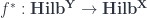
$f^* : \mathbf{Hilb^Y} \rightarrow \mathbf{Hilb^X}$

which comes from pulling back along $f$ – easiest to see for the MFHS, so that $f^*\mathcal{H}_x = \mathcal{H}_{f(x)}$ , and

$\int_f^{\oplus} : \mathbf{Hilb^X} \rightarrow \mathbf{Hilb^Y}$

the “direct image” operation, where in terms of MFHS, we have $(\int_f^{\oplus}\mathcal{H})_y = \int_{f^{-1}(y)}^{\oplus}\mathcal{H}_x d\mu_y(x)$ . That is, one direct-integrates over the preimage.

Now, these are measure-theoretic equivalents of two of the Grothendieck operations on sheaves (here is the text of Lipman’s Springer Lecture Notes book which includes an intro to them in Ch3 – a bit long for a first look, but the best I could find online). These are often discussed in the context of derived categories. The operation $\int_f^{\oplus}$ is the analog of what is usually called $f_*$ .

Part of what makes this different from the usual setting is that $\mathbf{Disint}$ is not as nice as $\mathbf{Top}$ , the more usual underlying category. What’s more, typically one talks about sheaves of sets, or abelian groups, or rings (which give the case of operations on schemes – i.e. topological spaces equipped with well-behaved sheaves of rings) – all of which are nicer categories than the category of Hilbert spaces. In particular, while in the usual picture $f_*$ is left adjoint to $f^*$ , this condition fails here because of the requirement that morphisms in $\mathbf{Hilb}$ are bounded linear maps – instead, there’s a unique extension property.

Similarly, while $f*$ is always defined by pulling back along a function $f$ , in the usual setting, the direct image functor $f_*$ is left-adjoint to $f^*$ , found by taking a left Kan extension along $f$ . This involves taking a colimit (specifically, imagine replacing the direct integral with a coproduct indexed over the same set). However, in this setting, the direct integral is not a coproduct (as the direct sum would be for vector spaces, or even finite-dimensional Hilbert spaces).

So in other words, something like the Grothendieck operations can be done with 2-Hilbert spaces, but the categorical properties (adjunction, Kan extension) are not as nice.

Finally, I’ll again remark that my motivation is to apply this to groupoids (or stacks), rather than just spaces $X$ , and thus build Extended TQFT’s from (compact) Lie groups – but that’s another story, as we said when I was young.

¹ Products: The fact that we want to look at spans in categories that aren’t Cartesian is the reason it’s more general to think about spans, rather than (as you can in some settings such as algebraic geometry) in terms of “bundles over the product”, which is otherwise equivalent. For sets or set-groupoids, this isn’t an issue.

October 27, 2009

“States” and Time – Hamiltonians, KMS states, and Tomita Flow

Posted by Jeffrey Morton under algebra, c*-algebras, musing, noncommutative geometry, philosophical, physics, quantum mechanics, reading
[11] Comments

When I made my previous two posts about ideas of “state”, one thing I was aiming at was to say something about the relationships between states and dynamics. The point here is that, although the idea of “state” is that it is intrinsically something like a snapshot capturing how things are at one instant in “time” (whatever that is), extrinsically, there’s more to the story. The “kinematics” of a physical theory consists of its collection of possible states. The “dynamics” consists of the regularities in how states change with time. Part of the point here is that these aren’t totally separate.

Just for one thing, in classical mechanics, the “state” includes time-derivatives of the quantities you know, and the dynamical laws tell you something about the second derivatives. This is true in both the Hamiltonian and Lagrangian formalism of dynamics. The Hamiltonian function, which represents the concept of “energy” in the context of a system, is based on a function $H(q,p)$ , where $q$ is a vector representing the values of some collection of variables describing the system (generalized position variables, in some configuration space $X$ ), and the $p = m \dot{q}$ are corresponding “momentum” variables, which are the other coordinates in a phase space which in simple cases is just the cotangent bundle $T*X$ . Here, $m$ refers to mass, or some equivalent. The familiar case of a moving point particle has “energy = kinetic + potential”, or $H = p^2 / m + V(q)$ for some potential function $V$ . The symplectic form on $T*X$ can then be used to define a path through any point, which describes the evolution of the system in time – notably, it conserves the energy $H$ . Then there’s the Lagrangian, which defines the “action” associated to a path, which comes from integrating some function $L(q, \dot{q})$ living on the tangent bundle $TX$ , over the path. The physically realized paths (classically) are critical points of the action, with respect to variations of the path.

This is all based on the view of a “state” as an element of a set (which happens to be a symplectic manifold like $T*X$ or just a manifold if it’s $TX$ ), and both the “energy” and the “action” are some kind of function on this set. A little extra structure (symplectic form, or measure on path space) turns these functions into a notion of dynamics. Now a function on the space of states is what an observable is: energy certainly is easy to envision this way, and action (though harder to define intuitively) counts as well.

But another view of states which I mentioned in that first post is the one that pertains to statistical mechanics, in which a state is actually a statisticial distribution on the set of “pure” states. This is rather like a function – it’s slightly more general, since a distribution can have point-masses, but any function gives a distribution if there’s a fixed measure $d\mu$ around to integrate against – then a function like $H$ becomes the measure $H d\mu$ . And this is where the notion of a Gibbs state comes from, though it’s slightly trickier. The idea is that the Gibbs state (in some circumstances called the Boltzmann distribution) is the state a system will end up in if it’s allowed to “thermalize” – it’s the maximum-entropy distribution for a given amount of energy in the specified system, at a given temperature $T$ . So, for instance, for a gas in a box, this describes how, at a given temperature, the kinetic energies of the particles are (probably) distributed. Up to a bunch of constants of proportionality, one expects that the weight given to a state (or region in state space) is just $exp(-H/T)$ , where $H$ is the Hamiltonian (energy) for that state. That is, the likelihood of being in a state is inversely proportional to the exponential of its energy – and higher temperature makes higher energy states more likely.

Now part of the point here is that, if you know the Gibbs state at temperature $T$ , you can work out the Hamiltonian
just by taking a logarithm – so specifying a Hamiltonian and specifying the corresponding Gibbs state are completely equivalent. But specifying a Hamiltonian (given some other structure) completely determines the dynamics of the system.

This is the classical version of the idea Carlo Rovelli calls “Thermal Time”, which I first encountered in his book “Quantum Gravity”, but also is summarized in Rovelli’s FQXi essay “Forget Time“, and described in more detail in this paper by Rovelli and Alain Connes. Mathematically, this involves the Tomita flow on von Neumann algebras (which Connes used to great effect in his work on the classification of same). It was reading “Forget Time” which originally got me thinking about making the series of posts about different notions of state.

Physically, remember, these are von Neumann algebras of operators on a quantum system, the self-adjoint ones being observables; states are linear functionals on such algebras. The equivalent of a Gibbs state – a thermal equilibrium state – is called a KMS (Kubo-Martin-Schwinger) state (for a particular Hamiltonian). It’s important that the KMS state depends on the Hamiltonian, which is to say the dynamics and the notion of time with respect to which the system will evolve. Given a notion of time flow, there is a notion of KMS state.

One interesting place where KMS states come up is in (general) relativistic thermodynamics. In particular, the effect called the Unruh Effect is an example (here I’m referencing Robert Wald’s book, “Quantum Field Theory in Curved Spacetime and Black Hole Thermodynamics”). Physically, the Unruh effect says the following. Suppose you’re in flat spacetime (described by Minkowski space), and an inertial (unaccelerated) observer sees it in a vacuum. Then an accelerated observer will see space as full of a bath of particles at some temperature related to the acceleration. Mathematically, a change of coordinates (acceleration) implies there’s a one-parameter family of automorphisms of the von Neumann algebra which describes the quantum field for particles. There’s also a (trivial) family for the unaccelerated observer, since the coordinate system is not changing. The Unruh effect in this language is the fact that a vacuum state relative to the time-flow for an unaccelerated observer is a KMS state relative to the time-flow for the accelerated observer (at some temperature related to the acceleration).

The KMS state for a von Neumann algebra with a given Hamiltonian operator has a density matrix $\omega$ , which is again, up to some constant factors, just the exponential of the Hamiltonian operator. (For pure states, $\omega = |\Psi \rangle \langle \Psi |$ , and in general a matrix becomes a state by $\omega(A) = Tr(A \omega)$ which for pure states is just the usual expectation value value for A, $\langle \Psi | A | \Psi \rangle$ ).

Now, things are a bit more complicated in the von Neumann algebra picture than the classical picture, but Tomita-Takesaki theory tells us that as in the classical world, the correspondence between dynamics and KMS states goes both ways: there is a flow – the Tomita flow – associated to any given state, with respect to which the state is a KMS state. By “flow” here, I mean a one-parameter family of automorphisms of the von Neumann algebra. In the Heisenberg formalism for quantum mechanics, this is just what time is (i.e. states remain the same, but the algebra of observables is deformed with time). The way you find it is as follows (and why this is right involves some operator algebra I find a bit mysterious):

First, get the algebra $\mathcal{A}$ acting on a Hilbert space $H$ , with a cyclic vector $\Psi$ (i.e. such that $\mathcal{A} \Psi$ is dense in $H$ – one way to get this is by the GNS representation, so that the state $\omega$ just acts on an operator $A$ by the expectation value at $\Psi$ , as above, so that the vector $\Psi$ is standing in, in the Hilbert space picture, for the state $\omega$ ). Then one can define an operator $S$ by the fact that, for any $A \in \mathcal{A}$ , one has

$(SA)\Psi = A^{\star}\Psi$

That is, $S$ acts like the conjugation operation on operators at $\Psi$ , which is enough to define $S$ since $\Psi$ is cyclic. This $S$ has a polar decomposition (analogous for operators to the polar form for complex numbers) of $S = J \Delta$ , where $J$ is antiunitary (this is conjugation, after all) and $\Delta$ is self-adjoint. We need the self-adjoint part, because the Tomita flow is a one-parameter family of automorphisms given by:

$\alpha_t(A) = \Delta^{-it} A \Delta^{it}$

An important fact for Connes’ classification of von Neumann algebras is that the Tomita flow is basically unique – that is, it’s unique up to an inner automorphism (i.e. a conjugation by some unitary operator – so in particular, if we’re talking about a relativistic physical theory, a change of coordinates giving a different $t$ parameter would be an example). So while there are different flows, they’re all “essentially” the same. There’s a unique notion of time flow if we reduce the algebra $\mathcal{A}$ to its cosets modulo inner automorphism. Now, in some cases, the Tomita flow consists entirely of inner automorphisms, and this reduction makes it disappear entirely (this happens in the finite-dimensional case, for instance). But in the general case this doesn’t happen, and the Connes-Rovelli paper summarizes this by saying that von Neumann algebras are “intrinsically dynamic objects”. So this is one interesting thing about the quantum view of states: there is a somewhat canonical notion of dynamics present just by virtue of the way states are described. In the classical world, this isn’t the case.

Now, Rovelli’s “Thermal Time” hypothesis is, basically, that the notion of time is a state-dependent one: instead of an independent variable, with respect to which other variables change, quantum mechanics (per Rovelli) makes predictions about correlations between different observed variables. More precisely, the hypothesis is that, given that we observe the world in some state, the right notion of time should just be the Tomita flow for that state. They claim that checking this for certain cosmological models, like the Friedman model, they get the usual notion of time flow. I have to admit, I have trouble grokking this idea as fundamental physics, because it seems like it’s implying that the universe (or any system in it we look at) is always, a priori, in thermal equilibrium, which seems wrong to me since it evidently isn’t. The Friedman model does assume an expanding universe in thermal equilibrium, but clearly we’re not in exactly that world. On the other hand, the Tomita flow is definitely there in the von Neumann algebra view of quantum mechanics and states, so possibly I’m misinterpreting the nature of the claim. Also, as applied to quantum gravity, a “state” perhaps should be read as a state for the whole spacetime geometry of the universe – which is presumably static – and then the apparent “time change” would then be a result of the Tomita flow on operators describing actual physical observables. But on this view, I’m not sure how to understand “thermal equilibrium”. So in the end, I don’t really know how to take the “Thermal Time Hypothesis” as physics.

In any case, the idea that the right notion of time should be state-dependent does make some intuitive sense. The only physically, empirically accessible referent for time is “what a clock measures”: in other words, there is some chosen system which we refer to whenever we say we’re “measuring time”. Different choices of system (that is, different clocks) will give different readings even if they happen to be moving together in an inertial frame – atomic clocks sitting side by side will still gradually drift out of sync. Even if “the system” means the whole universe, or just the gravitational field, clearly the notion of time even in General Relativity depends on the state of this system. If there is a non-state-dependent “god’s-eye view” of which variable is time, we don’t have empirical access to it. So while I can’t really assess this idea confidently, it does seem to be getting at something important.

October 3, 2008

Update. Curvature. 2-monads.

Posted by Jeffrey Morton under category theory, geometry, higher dimensional algebra, musing, reading, talks, tqft, update
[2] Comments

First off, a nice recent XKCD comic about height.

…

I’ve been busy of late starting up classes, working on a paper which should appear on the archive in a week or so on the groupoid/2-vector space stuff I wrote about last year. I resolved the issue I mentioned in a previous post on the subject, which isn’t fundamentally that complicated, but I had to disentangle some notation and learn some representation theory to get it figured out. I’ll maybe say something about that later, but right now I felt like making a little update. In the last few days I’ve also put together a little talk to give at Octoberfest in Montreal, where I’ll be this weekend. Montreal is a lovely city to visit, so that should be enjoyable.

A little while ago I had a talk with Dan’s new grad student – something for a class, I think – about classical and modern differential geometry, and the different ideas of curvature in the two settings. So the Gaussian curvature of a surface embedded in $\mathbb{R}^3$ has a very multivariable-calculus feel to it: you think of curves passing through a point, parametrized by arclength. The have a moving orthogonal frame attached: unit tangent vector, its derivative, and their cross-product. The derivative of the unit tangent is always orthogonal (it’s not changing length), so you can imagine it to be the radius of a circle, with length $r$ , the radius of curvature. Then you have $\kappa = \frac{1}{r}$ curvature along that path. At any given point on a surface, you get two degrees of freedom – locally, the curve looks like a hyperboloid or an ellipse, or whatever, so there’s actually a curvature form. The determinant gives the Gaussian curvature $K$ . So it’s a “second derivative” of the surface itself (if you think of it as ). The Gaussian curvature, unlike the curvature in particular directions, is intrinsic – preserved by isometry of the surface, so it’s not really dependent on the embedding. But this fact takes a little thinking to get to. Then there’s the trace – the scalar curvature.

In a Riemannian manifold, you need to have a connection to see what the curvature is about. Given a metric, there’s the associated Levi-Civita connection, and of course you’d get a metric on a surface embedded in $\mathbb{R}^3$ , inherited from the ambient space. But the modern point of view is that the connection is the important object: the ambient space goes away entirely. Then you have to think of what the curvature represents differenly, since there’s no normal vector to the surface any more. So now we’re assuming we want an intrinsic version of the “second derivative of the surface” (or n-manifold) from the get-go. Here you look at the second derivative of the connection in any given coordinate system. You’re finding the infinitesimal noncommutativity of parallel transport w.r.t two coordinate directions: take a given vector, and transport it two ways around an infinitesimal square, and take the difference, get a new vector. This all is written as a (3,1)-form, the Riemann tensor. Then you can contract it down and get a matrix again, and then contract on the last two indices (a trace!) and you get back the scalar curvature again – but this is all in terms of the connection (the coordinate dependence all disappears once you take the trace).

I hadn’t thought about this stuff in coordinates for a while, so it was interesting to go back and work through it again.

In the noncommutative geometry seminar, we’ve been talking about classical mechanics – the Lagrangian and Hamiltonian formulation. So it reminded me of the intuition that curvature – a kind of second derivative – often shows up in Lagrangians for field theories using connections because it’s analogous to kinetic energy. A typical mechanics Lagrangian is something like (kinetic energy) – (potential energy), but this doesn’t appear much in the topological field theories I’ve been thinking about because their curvature is, by definition, zero. Topological field theory is kind of like statics, as opposed to mechanics, that way. But that’s a handy simplification for the program of trying to categorify everything. Since the whole space of connections is infinite dimensional, worrying about categorified action principles opens up a can of worms anyway.

So it’s also been interesting to remember some of that stuff and discuss it in the seminar – and it was inially suprising that it’s the introduction to “noncommutative geometry”. It does make sense, though, since that’s related to the formalism of quantum mechanics: operator algebras on Hilbert spaces.

Finally, I was looking for something on 2-monads for various reasons, and found a paper by Steve Lack which I wanted to link to here so I don’t forget it.

The reason I was looking was that (a) Enxin Wu, after talking about deformation theory of algebras, was asking after monads and the bar construction, which we talked about at the UCR “quantum gravity” seminar, so at some point we’ll take a look at that stuff. But it reminded me that I was interested in the higher-categorical version of monads for a different reason. Namely, I’d been talking to Jamie Vicary about his categorical description of the harmonic oscillator, which is based on having a monad in a nice kind of monoidal category. Since my own category-theoretic look at the harmonic oscillator fits better with this groupoid/2-vector space program I’ll be talking about at Octoberfest (and posting about a little later), it seemed reasonable to look at a categorified version of the same picture.

But first things first: figuring out what the heck a 2-monad is supposed to be. So I’ll eventually read up on that, and maybe post a little blurb here, at some point.

Anyway, that update turned out to be longer than I thought it would be.

September 15, 2008

Arrow’s Theorem, Strategic Voting etc.

Posted by Jeffrey Morton under musing, reading
[11] Comments

I mentioned before that I wanted to try expanding the range of things I blog about here. One example is that I have a long-standing interest in game theory, which I think began when I was an undergrad at U of Waterloo. I don’t (currently) do research in game theory, and have nothing particularly novel to say about it (though naturally a default question for me would be: can you categorify it?), but it is regularly used to analyze situations in evolutionary theory, and social sciences like economics, and politics. So it seems to be a fairly fundamental discipline, and worth looking at, I think.

For a little over a week now, Canada has been in a campaign leading up to a federal election in October. Together with the constant coverage of the US election campaign, this means the news is full of politicking, projections of results, etc. Also as usual, there are less-well-covered people agitating for electoral reform. So it seemed as good a time as any to blog something about social choice theory, which is an application of game theory to the special problem of making choices in groups which reflect the preferences of its members.

This is the defining problem for democracy, which is (in recent times) the world’s most popular political system, so it has been pretty extensively studied. One aspect of democracy is voting. One aspect of social choice theory is the study of voting systems – algorithms which collect information about the populations preferences among some alternatives, and produce a “social choice function”. For example, the US Presidential election process (in its ideal form, and excluding Primaries) collects the name of one candidate from each voter, and returns the name of a single winner. The Australian process collects more information from each voter: an ordered list of candidates. It uses a variant of the voting scheme called STV, which can return more than one winner.

Okay, so there are many different voting methods. Why should there be so many? Why not just use the best? For one thing, there are different criteria what is meant by “best”, and every voting system has some sort of limitation. Depending on your precise criteria, you may prefer one system or another. A more precise statement of this comes in the form of Arrow’s theorem.

Suppose we have a set $C$ of “choices” (a general term for alternatives, not necessarily candidates for office), and for each voter $v$ in the population of voters $V$ , there is $P_v$ , a total order on $C$ (a “preference order”). Call this information a “profile”. Then we’d like to collect some information about the profile (perhaps the whole thing, perhaps not), and produce a “social preference order” $P$ . This is a function $c : \mathcal{O}(C)^V \rightarrow \mathcal{O}(C)$ (where $\mathcal{O}(C)$ is the set of orders on $C$ ). The functon $c$ should satisfy some conditions, of course, and many possible conditions have been defined. Arrow’s theorem is usually stated with five conditions, but an equivalent form uses these:

Unrestricted Domain: $c$ is surjective. (I.e. any preference order could potentially occur as output of the algorithm – e.g. in a single-winner election, the system should allow any candidate to win, given enough votes)
Independence of Irrelevant Alternatives: for any $S \subset C$ , the restriction $c\|_{S} : \mathcal{O}(S)^V \rightarrow \mathcal{O}(S)$ agrees with $c$ (i.e. when applied to the restrictions of the orders $P_v$ to $S$ , it produces the restriction of $P$ to $S$ . In particular, removing a non-winning candidate from the ballot should not affect the outcome.)
Monotonicity: if $P$ prefers alternative $a$ to $b$ , then changing any $P_v$ so that it prefers $a$ to $b$ (assuming it did not) should not cause $P$ to prefer $b$ to $a$ (i.e. no voter’s ballot has a harmful effect on their preferred candidate).

Arrow’s theorem says that no algorithm satisfies all three conditions (and of course some algorithms don’t satisfy any). (A different formulation and its proof can be found here.)

Most popular voting systems satisfy (1) and (3) since these are fairly obvious criteria of fairness: every candidate has a chance, and nobody’s votes have negative weight (though note that a popular reform suggestion in the US, Instant Runoff Voting, fails monotonicity!). Condition (2) is the one that most people seem to find non-obvious. Failures of condition (2) can take various forms. One is “path dependence”, which may occur if the decision is made through a number of votes, and the winner can (for some profiles) depend on the order in which the votes are taken (for instance, the runoff voting used in French presidential elections is path dependent). When a voting system has this property, the outcome can sometimes be manipulated by the “agenda-setter” (if there is one).

Another way (2) can fail is by creating the possibility of strategic voting: creating a situation in which voters have a rational incentive to give false information about their preferences. For instance, voters may want to avoid “splitting” the vote. In the US election in 2000, the presence of the “irrelevant” (i.e. non-winning) alternative Ralph Nader (allegedly) split the vote which otherwise would have gone to Gore, allowing Bush to win certain states. Somewhat similarly, in the current Canadian election, there is a single “right wing” party (Conservative), two or three “left wing” parties, depending on the riding (Liberal, NDP, Bloc Quebecois), and one which is neither (Green). In some competitive districts, for example, voters who prefer NDP to Liberal, but Liberal to Conservative, have a rational reason to vote for their second choice in order to avoid their third choice – assuming they know the “real” race is between Conservative and Liberal in their riding. (In my riding, North London Centre, this is not an issue since the outcome – Liberal – is not in doubt at all.)

These, like all voting system flaws, only become apparent when there are at least three options: with only two options, condition (2) doesn’t apply, since removing one option leaves nothing to vote on. (This is one reason why many voting systems are said to “favour the two-party system”, where its flaws are not apparent: when the vote is split, voters have an incentive to encourage parties to merge. This is why Canada now has only one “right-wing” party).

These two flaws also allow manipulation of the vote only when the manipulator knows enough about the profile of preferences. Apart from allowing parties to find key competitive ridings (or states, etc.), this is probably one of the most important uses of polling data. (Strategic voting is hard in Canada, since a good statistical sample of, say, 1000 in each of 308 ridings would require polling about 1% of the total population of the country, so one usually has only very imperfect information about the profile. Surveying 1000 people in each of 50 US states is relatively much easier. Even at that, projections are hard: try reading any of the methodology details on, say, fivethirtyeight.com for illustration.)

Now, speaking of strategic voting, the Gibbard-Satterthwaite theorem, closely related to Arrow’s theorem, applies to social choice systems which aim to select a single winner based on a number of votes. (Arrow’s theorem originally doesn’t specifically apply to voting: it applies to any multi-criterion decision-making process). The G-S theorem says that any (deterministic) voting system satisfies one of three conditions:

It is dictatorial (i.e. there is a voter $v$ such that the winner depends only on $P_v$
It is restricted (i.e. there is some candidate who cannot win no matter the profile)
It allows strategic voting for some profiles

So it would seem that the possibility of strategic voting can’t reasonably be done away with. This suggests the point of view that voting strategically is no more a problem than, say, playing chess strategically. The fact that an analysis of voting in terms of the theory of games of strategy suggests this point of view is probably not a coincidence…

As I remarked, here in London North Centre, the outcome of the vote is in no doubt, so, strategically speaking, any vote is as good as any other, or none. This curious statement is, paradoxically, only true if not believed by most voters – voting strategically in a context where other voters are doing the same, or worse yet, answering pollsters strategically, is a much more complicated game with incomplete (and unreliable) information. This sort of thing is probably why electoral reform is a persistent issue in Canada.

June 28, 2008

20th Century Space and 10th Century Space

Posted by Jeffrey Morton under c*-algebras, historical, noncommutative geometry, philosophical, physics, reading
[2] Comments

A couple of posts ago, I mentioned Max Jammer’s book “Concepts of Space” as a nice genealogy of that concept, with one shortcoming from my point of view – namely, as the subtitle suggests, it’s a “History of Theories of Space in Physics”, and since physics tends to use concepts out of mathematics, it lags a bit – at least as regards fundamental concepts. Riemannian geometry predates Einstein’s use of it in General Relativity by fifty some years, for example. Heisenberg reinvented matrices and matrix multiplication (which eventually led to wholesale importation of group theory and representation theory into physics). More examples no doubt could be found (String Theory purports to be a counterexample, though opinions differ as to whether it is real physics, or “merely” important mathematics; until it starts interacting with experiments, I’m inclined to the latter, though of course contra Hardy, all important mathematics eventually becomes useful for something).

What I said was that it would be nice to see further investigation of concepts of space within mathematics, in particular Grothendieck’s and Connes’. Well, in a different context I was referred to this survey paper by Pierre Cartier from a few years back, “A Mad Day’s Work: From Grothendieck To Connes And Kontsevich, The Evolution Of Concepts Of Space And Symmetry”, which does at least some of that – it’s a fairly big-picture review that touches on the relationship between these new ideas of space. It follows that stream of the story of space up to the end of the 20th century or so.

There’s also a little historical/biographical note on Alexander Grothendieck – the historical context is nice to see (one of the appealing things about Jammer’s book). In this case, much of the interesting detail is more relevant if you find recent European political history interesting – but I do, so that’s okay. In fact, I think it’s helpful – maybe not mathematically, but in other ways – to understand the development of mathematical ideas in the context of history. This view seems to be better received the more ancient the history in question.

On the scientific end, Cartier tries to explain Grothendieck’s point of view of space – in particular what we now call topos theory – and how it developed, as well as how it relates to Connes’. Pleasantly enough, a key link between them turns out to be groupoids! However, I’ll pass on commenting on that at the moment.

…

Instead, let me take a bit of a tangent and jump back to Jammer’s book. I’ll tell you something from his chapter “Emancipation from Aristotelianism” which I found intriguing. This would be an atomistic theory of space – an idea that’s now beginning to make something of a comeback, in the guise of some of the efforts toward a quantum theory of gravity (EDIT: but see comments below). Loop quantum gravity, for example, deals with space in terms of observables, which happen to take the form of holonomies of connections around loops. Some of these observables have interpretations in terms of lengths, areas, and volumes. It’s a prediction of LQG that these measurements should have “quantized”, which is to say integer, values: states of LQG are “spin networks”, which is to say graphs with (quantized) labels on the edges, interpreted as areas (in a dual cell complex). (Notice this is yet again another, different, view of space, different from Grothendieck’s or Connes’, but shares with Connes especially the idea of probing space in some empirical way. Grothendieck “probes” space mainly via cohomology – how “empirical” that is depends on your point of view.)

The atomistic theory of space Jammer talks about is very different, but it does also come from trying to reconcile a discrete “quantum” theory of matter with a theory linking matter to space. In particular, the medieval Muslim philosophical school known as al Kalam tried to reconcile the Koran and Islamic theology with Greek philosophy (most of the “Hellenistic” world conquered by Alexander the Great, not least Egypt, is inside Dar al Islam, which is why many important Greek texts came into Europe via Arabic translations). Though they were, as Jammer says, “Emancipating” themselves from Aristotle, they did share some of his ideas about space.

For Aristotle, space meant “place” – the answer to the questions “where is it?” and “what is its shape and size?”. In particular, it was first and foremost an attribute of some substance. All “where?” questions are about some THING. The answer is defined in terms of other things: my cat is on the ground, under the tree, beside the house. The “place” of an object was literally the inner shell of the containing body that held it (which was contained by some other body, and so on – there being no vacuum in Aristotle). So my “place” is defined by (depending how you look at it) my skin, my clothes, or the walls of the room I’m in. This is a relational view of space, though more hard-headed than, say, Leibniz’s.

The philosophers of the Kalam had a similar relational view of space, but they didn’t accept Aristotle’s view of “substances”, where each thing has its own essential identity, on which attributes are hung like hats. Instead, they believed in atomism, following Democritus and Leucippus: bodies were made out of little indivisible nuggets called “atoms”. Macroscopic things were composites of atoms, and their attributes resulted from how the atoms were put together. Here’s Jammer’s description:

The atoms of the Kalam are indivisible particles, equal to each other and devoid of all extension. Spatial magnitude can be attributed only to a combination of atoms forming a body. Although a definite position (hayyiz) belongs to each individual atom, it does not occupy space (makan). It is rather the set of these positions – one is almost tempted to say, the system of relations – that constitutes spatial extension….

In the Kalam, these rather complicated and surprisingly abstract ideas were deemed necessary in order to meet Aristotle’s objections against atomism on the ground that a spatial continuum cannot be constituted by, or resolved into, indivisibles nor can two points be continuous or contiguous with one another.

So like people who prefer a “background independent” quantum theory of gravity, they wanted to believe that space (geometry) derives from matter, and that matter is discrete, but space was commonly held to be continuous. Also alike, they resolved the problem by discarding the assumption of continuous space, and, by consideration of motion, to discrete time.

There are some differences, though. The most obvious is that the nodes of the graph in a spin network state don’t represent units of matter, or “atoms”. For that matter, quantum field theory doesn’t really have “atoms” in the sense of indivisible units which don’t break apart or interact. Everything interacts in QFT. (In some sense, interactions are more fundamental units in QFT than “particles” are – particles only (sic!) serve to connect one interaction with another.)

Another key difference is how space relates to matter. In Aristotle, and in the Kalam, space is defined directly by matter: two bits of matter “define” the space between them. In General Relativity (the modern theory with the “relational” view of space), there’s still room for space as an actor in its own right, like Newton’s absolute space-as-independent-variable – in other words, room for a vacuum, which Aristotle categorically denied could even conceivably exist. In GR, what matter determines is the curvature of space (more precisely the Einstein tensor of the curvature).

Well, so the differences are probably more informative than the similarities,

(Edit: To emphasize a key difference glossed over before… It was coupling to quantum matter which suggested quantizing the picture of space. Discreteness of the spectrum of various observables is a logically separate prediction in each case. Either matter or space(time) could have had continuous spectrum for the relevant observables and still been quantized – discrete matter would have given discreteness for some observed quantities, but not area, length, and so on. So in the modern setting, the link is much less direct.)

but the fact that theories of related discreteness in matter, space, and time, have been around for a thousand years or more is intriguing. The idea of empty space as an independent entity – in the modern form only about three hundred years old – appears to be the real novel part. One of the nice intuitions in Carlo Rovelli’s book on Quantum Gravity, for me at least, was to say that, rather than there being a separate “space”, we have a theory of fields defined on other fields as background – one of which, the “gravitational field” has customarily been taken for “space”. So spatial geometry is a field, and it has some propagating (through space!) degrees of freedom – the particle associated to this field is a graviton. Nobody’s ever seen one, mind you – but supposing they exist makes many of things easier.

To re-state a previous point: I think this is a nice aspect of categorification for dealing with space. Extending the “stuff/structure/properties” trichotomy to allow space to resemble both “stuff” and relations between stuff leaves room for both points of view.

…

I mention this because tomorrow I leave London (Ontario) for London (England), and thence to Nottingham, for the Quantum Gravity and Quantum Geometry Conference. It’s been a while since I worked much on quantum gravity, per se, but this conference should be interesting because it seems to be a confluence of mathematically and physically inclined people, as the name suggests. I read on the program, for example, that Jerzy Lewandowski is speaking on QFT in Quantum Curved Spacetime, and suddenly remember that, oh yes, I did a Masters thesis (viz) on QFT in curved (classical) spacetime… but that was back in the 20th century!

It’s been a while, and I only made a small start at it before, but that whole area of physics is quite pretty. Anyway, it should be interesting, and there are a number of people I’m looking forward to talking to.

May 28, 2008

Correspondences and Spans

Posted by Jeffrey Morton under c*-algebras, category theory, noncommutative geometry, philosophical, quantum mechanics, reading, spans
[2] Comments

In the past couple of weeks, Masoud Khalkhali and I have been reading and discussing this paper by Marcolli and Al-Yasry. Along the way, I’ve been explaining some things I know about bicategories, spans, cospans and cobordisms, and so on, while Masoud has been explaining to me some of the basic ideas of noncommutative geometry, and (today) K-theory and cyclic cohomology. I find the paper pretty interesting, especially with a bit of that background help to identify and understand the main points. Noncommutative geometry is fairly new to me, but a lot of the material that goes into it turns out to be familiar stuff bearing unfamiliar names, or looked at in a somewhat different way than the one I’m accustomed to. For example, as I mentioned when I went to the Groupoidfest conference, there’s a theme in NCG involving groupoids, and algebras of $\mathbb{C}$ -linear combinations of “elements” in a groupoid. But these “elements” are actually morphisms, and this picture is commonly drawn without objects at all. I’ve mentioned before some ideas for how to deal with this (roughly: $\mathbb{C}$ is easy to confuse with the algebra of $1 \times 1$ matrices over $\mathbb{C}$ ), but anything special I have to say about that is something I’ll hide under my hat for the moment.

I must say that, though some aspects of how people talk about it, like the one I just mentioned, seem a bit off, to my mind, I like NCG in many respects. One is the way it ties in to ideas I know a bit about from the physics end of things, such as algebras of operators on Hilbert spaces. People talk about Hamiltonians, concepts of time-evolution, creation and annihilation operators, and so on in the algebras that are supposed to represent spaces. I don’t yet understand how this all fits together, but it’s definitely appealing.

Another good thing about NCG is the clever elegance of Connes’ original idea of yet another way to generalize the concept “space”. Namely, there was already a duality between spaces (in the usual sense) and commutative algebras (of functions on spaces), so generalizing to noncommutative algebras should give corresponding concepts of “spaces” which are different from all the usual ones in fairly profound ways. I’m assured, though I don’t really know how it all works, that one can do all sorts of things with these “spaces”, such as finding their volumes, defining derivatives of functions on them, and so on. They do lack some qualities traditionally associated with space – for instance, many of them don’t have many, or in some cases any, points. But then, “point” is a dubious concept to begin with, if you want a framework for physics – nobody’s ever seen one, physically, and it’s not clear to me what seeing one would consist of…

(As an aside – this is different from other versions of “pointless” topology, such as the passage from ordinary topologies to, sites in the sense of Grothendieck. The notion of “space” went through some fairly serious mutations during the 20th century: from Einstein’s two theories of relativity, to these and other mathematicians’ generalizations, the concept of “space” has turned out to be either very problematic, or wonderfully flexible. A neat book is Max Jammer’s “Concepts of Space“: though it focuses on physics and stops in the 1930’s, you get to appreciate how this concept gradually came together out of folk concepts, went through several very different stages, and in the 20th century started to be warped out of all recognition. It’s as if – to adapt Dan Dennett – “their word for milk became our word for health”.I would like to see a comparable history of mathematicians’ more various concepts, covering more of the 20th century. Plus, one could probably write a less Eurocentric genealogy nowadays than Jammer did in 1954.)

Anyway, what I’d like to say about the Marcolli and Al-Yasry paper at the moment has to do with the setup, rather than the later parts, which are also interesting. This has to do with the idea of a correspondence between noncommutative spaces. Masoud explained to me that, related to the matter of not having many points, such “spaces” also tend to be short on honest-to-goodness maps between them. Instead, it seems that people often use correspondences. Using that duality to replace spaces with algebras, a recurring idea is to think of a category where morphism from algebra $A$ to algebra $B$ is not a map, but a left-right $(A,B)$ -bimodule, $_AM_B$ . This is similar to the business of making categories of spans.

Let me describe briefly what Marcolli and Al-Yasry describe in the paper. They actually have a 2-category. It has:

Objects: An object is a copy of the 3-sphere $S^3$ with an embedded graph $G$ .

Morphisms: A morphism is a span of branched covers of 3-manifolds over $S^3$ :

$G_1 \subset S^3 \stackrel{\pi_1}{\longleftarrow} M \stackrel{\pi_2}{\longrightarrow} S^3 \supset G_2$

such that each of the maps $\pi_i$ is branched over a graph containing $G_i$ (perhaps strictly). In fact, as they point out, there’s a theorem (due to Alexander) proving that ANY 3-manifold $M$ can be realized as a branched cover over the 3-sphere, branched at some graph (though perhaps not including a given $G$ , and certainly not uniquely).

2-Morphisms: A 2-morphism between morphisms $M_1$ and $M_2$ (together with their $\pi$ maps) is a cobordism $M_1 \rightarrow W \leftarrow M_2$ , in a way that’s compatible with the structure of the $lateux M_i$ as branched covers of the 3-sphere. The $M_i$ are being included as components of the boundary $\partial W$ – I’m writing it this way to emphasize that a cobordism is a kind of cospan. Here, it’s a cospan between spans.

This is somewhat familiar to me, though I’d been thinking mostly about examples of cospans between cospans – in fact, thinking of both as cobordisms. From a categorical point of view, this is very similar, except that with spans you compose not by gluing along a shared boundary, but taking a fibred product over one of the objects (in this case, one of the spheres). Abstractly, these are dual – one is a pushout, and the other is a pullback – but in practice, they look quite different.

However, this higher-categorical stuff can be put aside temporarily – they get back to it later, but to start with, they just collapse all the $hom$ -categories into $hom$ -sets by taking morphisms to be connected components of the categories. That is, they think about taking morphisms to be cobordism classes of manifolds (in a setting where both manifolds and cobordisms have some branched-covering information hanging around that needs to be respected – they’re supposed to be morphisms, after all).

So the result is a category. Because they’re writing for noncommutative geometry people, who are happy with the word “groupoid” but not “category”, they actually call it a “semigroupoid” – but as they point out, “semigroupoid” is essentially a synonym for (small) “category”.

Apparently it’s quite common in NCG to do certain things with groupoids $\mathcal{G}$ – like taking the groupoid algebra $\mathbb{C}[\mathcal{G}]$ of $\mathbb{C}$ -linear combinations of morphisms, with a product that comes from multiplying coefficients and composing morphisms whenever possible. The corresponding general thing is a categorical algebra. There are several quantum-mechanical-flavoured things that can be done with it. One is to let it act as an algebra of operators on a Hilbert space.

This is, again, a fairly standard business. The way it works is to define a Hilbert space $\mathcal{H}(G)$ at each object $G$ of the category, which has a basis consisting of all morphisms whose source is $G$ . Then the algebra acts on this, since any morphism $M'$ which can be post-composed with one $M$ starting at $G$ acts (by composition) to give a new morphism $M' \circ M$ starting at $G$ – that is, it acts on basis elements of $\mathcal{H}(G)$ to give new ones. Extending linearly, algebra elements (combinations of morphisms) also act on $\mathcal{H}(G)$ .

So this gives, at each object $G$ , an algebra of operators acting on a Hilbert space $\mathcal{H}(G)$ – the main components of a noncommutative space (actually, these need to be defined by a spectral triple: the missing ingredient in this description is a special Dirac operator). Furthermore, the morphisms (which in this case are, remember, given by those spans of branched covers) give correspondences between these.

Anyway, I don’t really grasp the big picture this fits into, but reading this paper with Masoud is interesting. It ties into a number of things I’ve already thought about, but also suggests all sorts of connections with other topics and opportunities to learn some new ideas. That’s nice, because although I still have plenty of work to do getting papers written up on work already done, I was starting to feel a little bit narrowly focused.

Theoretical Atlas