Thoughts on Philosophy of Contemporary Mathematics – II

This is the second post of my thoughts inspired mainly by reading Fernando Zalamea’s “Synthetic Philosophy of Contemporary Mathematics” (and also a few other sources). The first part is here.

I do have a few issues with the Zalamea book: mainly, as a reader, pinning down what a lot of the sentences really mean can be hard. This might be a combination perfectly reasonable things: the fact that it’s doing philosophy  – and it’s not analytic philosophy, which aspires to math-like rigour. (Indeed, one of the many ideas the book throws around is that of “synthetic philosophy”, modelled not after formal logic, but sheaf theory, with many local points of view and ways of relating them in areas where they overlap. Intuitively appealing, though it’s hard to see how to make it rigorous in the same way.)

So, many of the ideas are still formative, and the terms used to describe them are sometimes new coinages. Then, too, the combination of philosophical jargon and the fact that it’s translated from Spanish probably contribute. So I give the author the benefit of the doubt on this point and interpret the best I can. Even so, it’s still difficult for me to say exactly what some of it is saying. In any case, here I wanted to break down my understanding of some themes it is pointing out. There is more there than I have space to deal with here, but these are some major ones.

I had a somewhat similar response to David Corfield’s book, “Toward a Philosophy of Real Mathematics” (which Zalamea mentions in a chapter where he acknowledges some authors who have engaged the kind of issues he’s interested in). That is, both of them do well at pointing out topics which haven’t received much attention, but the main strength is by pointing out areas of actual mathematical activity, and describing what they’re like (for example, Corfield’s chapter on higher category theory, and Zalamea’s account of Grothendieck’s work). They both feel sort of preliminary, though, in that they’re pointing out areas where a lot more people need to study, argue, and generally thrash out various positions on the issues before (at least as far as I can see) one could hope to say the issues raised have actually been dealt with.

Themes

In any case, part of the point is that for a philosophical take on what mathematicians are actually studying, we need to look at some details. In the previous post I outlined the summary (from philosopher Albert Lautman) of the themes of “Elementary” and “Classical” mathematics. Lautman introduced five themes apropos to the “Modern” period – characterizing what was new compared to the “Classical” (say, pre-1900 or so). Zalamea’s claim, which seems correct to me, is that all of these themes are still present today, but some new ones have been added.

That is, mathematics is cumulative: all the qualities from previous periods stay important, but as it develops, new aspects of mathematics become visible. Thus, Lautman had five points, which are somewhat detailed, but the stand-out points to my mind include:

The existence of a great many different axiomatic systems and theories, which are not reducible to each other, but are related in various ways . Think of the profusion of different algebraic gadgets, such as groups, rings, quandles, magmas, and so on, each of which has its own particular flavour. Whereas Classical mathematics did a lot with, say, the real number system, the Modern period not only invented a bunch of other number systems and algebras, but also a range of different axiom systems for describing different generalizations. The same could be said in analysis: the work on the Calculus in the Classical period leads into the definition of a metric space and then a topological space in the Modern period, and an increasing profusion of specific classes of them with different properties (think of all the various separation axioms, for example, and the web of implications relating them).

The study of a rich class of examples of different axiomatic systems. Here the standout example to me is the classification of the finite groups, where the “semantics” of the classification is much more complex than the “syntax” of the theory. This reminds me of the game of Go (a.k.a. Wei Chi in China, or Baduk in Korea), which has gained some recent fame because of the famous AlphaGo victories. The analogy: that the rules of the game are very simple, but the actual practice of play is very difficult to master, and the variety of examples of games is huge. This is, essentially, because of a combinatorial explosion, and somewhat the same principle is at work in mathematics: the theory of groups has, essentially, just three axioms on one set with three structures (the unit, the inverse, and the multiplication – a 0-ary, unary, and binary operation respectively), so the theory is quite simple. Yet the classification of all the examples is complicated and full of lots of exceptions (like the sporadic simple groups), to the point that it was only finished in Contemporary times. Similar things could be said about topological spaces.

A unity of methods beyond apparent variety. An example cited being the connection between the Galois group of field extensions and the group of deck transformations of a certain kind of branched cover of spaces. In either case, the idea is to study a mathematical object by way of its group of automorphisms over some fixed base object – and in particular to classify intermediate objects by way of the subgroups of this big group. Here, the “base object” could refer to either a sub-field (which is a sub-object in the category of fields) or a base space for the cover (which is not – it’s a quotient, or more generically the target of a projection morphism). These are conceptually different kinds of things on the face of it, but the mechanism of studying “homomorphisms over” them is similar. In fact, following through the comparison reveals a unification, by considering the fields of functions on the spaces: a covering space then has a function field which is an extension of the base case, and the two apparently different situations turn out to correspond exactly.

A “dialectical movement that is a back-and-forth between the One and the Many”. This is one of those jargon-sounding terms (especially the Hegelian-sounding term “dialectic”) and is a bit abstract. The examples given include:

• The way multiple variants on some idea are thought up, which in turn get unified into a more general theory, which in turn spawns its own variants, and so on. So, as people study different axiom systems for set theory, and their models, this diversity gets unified into the study of the general principles of how such systems all fit together. That is, as “meta-mathematics”, which considers which models satisfy a given theorem, which axioms are required to prove it, etc.
• The way branches of mathematics (algebra, geometry, analysis, etc.) diverge and develop their own distinct characters, only to be re-unified by mixing them together in new subjects: algebraic geometry, analytic number theory, geometric analysis, etc. intil they again seem like parts of a big interrelated whole. Beyond these obvious cases, the supposedly different sub-disciplines develop distinctive ideas, tools, and methods, but then borrow them from each other as fast as they specialize. This back-and-forth between specialization and cross-fertilization is thus an example of “dialectic”.

Zalamea suggests that in the Contemporary period, all these themes are still present, but that some new ones have become important as well:

“Structural Impurity of Arithmetic” – this is related to subjects outside my range of experience, like the Weil Conjectures and the Langlands Program, so I don’t have much to say about it, except to note that, by way of arithmetic functions like zeta functions, they relate number theory to algebraic curves and geometry, and constitute a huge research program that came into being in the Contemporary period (specifically the late 1960’s and early 1970’s). (Edward Frenkel described the Langlands program as “a kind of grand unified theory of mathematics” for this among other reasons.)

Geometrization of Mathematics – essentially, the migration of tools and methods originally developed for like the way topos theory turns logic into a kind of geometry in which the topology of a space provides the algebra of possible truth values. This feeds into the pervasive use of sheaves in modern mathematics, etc. Or, again, the whole field of noncommutative geometry, geometric ideas about space are interpreted as  (necessarily commutative) algebra of functions on that space with pointwise multiplication: differential operators like the Lagrangian, for instance, capture metric geometry, while bundles over a space have an interpretation in terms of modules over the algebra. These geometric concepts can be applied to noncommutative algebras , thus treating them as if they were spaces.

“Schematization”, and becoming detached from foundations: in particular, the idea that what it means to study, for instance, “groups” is best understood in terms of the properties of the category of groups, and that an equivalent category, where the objects have some different construction, is just as good. You see this especially in the world of -categories: there are many different definitions for the entities being studied, and there’s increasingly an attitude that we don’t really need to make a specific choice. The “homotopy hypotesis” for -groupoids is an example of this: as long as these form a model of homotopy types, and their collectivity is a “homotopy theory” (with weak equivalences, fibrations, etc.) that’s homotopy-equivalent to the corresponding structure you get from another definition, they are in some sense “the same” idea. The subject of Univalent Foundations makes this very explicit.

“Fluxion and Deformation” of the boundaries of some previously fixed subject. “Fluxion” is one of those bits of jargon-sounding words which is suggestive, but I’m not entirely clear if it has a precise measing. This gets at the whole area of deformation theory, quantization (in all its various guises), and so on. That is, what’s happening here is that previously-understood structures which seemed to be discrete come to be understood as points on a continuum. Thus, for instance, we have -deformation: this starts a bit earlier than the Contemporary period, with the -integers, which are really power series in a variable , which just amount to the integers they’re deformations of when has the value 1. It really takes off later with the whole area of -deformations of algebra – in which such power series take on the role of the base ring.  Both of these have been studied by people interested in quantum physics, where the parameter , or the commutators in are pegged to the Planck constant .

There’s also reflexivity of modern mathematics, theories applied to themselves. This is another one of those cases where it’s less clear to me what the term is meant to suggest (though examples given include fixed point theorems and classification theorems.)

There’s a list near the beginning of notable mathematicians who illustrate

Zalamea synthesizes these into three big trends described with newly coined terms: “eidal“, “quiddital“, and “archaeal” mathematics. He recognizes these are just convenient rules of thumb for characterizing broad aspects of contemporary research, rather than rigorously definable ideas or subfields. This is a part of the book which I find more opaque than the rest – but essentially the distinction seems to be as follows.

Roughly, eidal mathematics (from the Greek eidos or “idea”) seems to describe the kind that involves moving toward the abstract, and linking apparently unrelated fields of study. One big example referenced here is the Langlands program, which is a bunch of conjectures connecting number theory to geometry. Also under this umbrella he references category theory, especially via Lawvere, which subsumes many different fields into a common framework – each being the study of some particular category such as Top, perhaps by relating it to some other category (such as, in algebraic topology, Grp).

The new term quiddital mathematics (from Latin quidditas, “what exists” or literally “whatness”) appears to refer to the sort which is intimately connected to physics. The way ideas that originate in physics have driven mathematics isn’t totally new: Calculus is a classical example. But more recently, the study of operator algebras was driven by quantum mechanics, index theory which links differential operators and topology was driven by quantum field theory, and there’s a whole plethora of mathematics that has grown out of String Theory, CFT, TQFT, and so forth – which may or may not turn out to be real physics, but were certainly inspired by theorizing about it. And, while it hasn’t had as deep an effect on pure mathematics, as far as I know, I imagine this category would include those areas of study that arose out of other applied studies, such as the theory of networks or the dynamics of large complex systems.

The third new coinage, archaeal mathematics (from arche, or “origin”, also giving the word “archetype”) is another one whose meaning is harder for me to pin down, because the explanation is quite abstract. In the structure of the explanation, this seems to be playing a role that mediates between the first two: something that mediates moving between very abstract notions and concrete realizations of them. One essential idea here is the finding of “invariants”, though what this really seems to mean is more like finding a universal structure of a given type. A simple case might be that between the axioms of groups, and particular examples that show up in practice, we might have various free groups – they’re concrete but pure examples of the theory, and other examples come from imposing more relations on them.

I’m not entirely sure about these three categories, but I do think there’s a good point here. This is that there’s a move away from the specifics and toward general principles. The huge repertoire of “contemparary” mathematics can be sort of overwhelming, and highly detailed. The five themes listed by Lautman, or Zalamea’s additional five, are an attempt to find trends, or deal descriptively with that repertoire. But it’s still, in some ways, a taxonomy: a list of features. Reducing the scheme to these three, whether this particular system makes sense to you or not, is more philosophical: rather than giving a taxonomy, it’s an effort to find underlying reasons why these themes and not others are generating the mathematics we’re doing.  So, while I’m not completely convinced about this system as an account of what contemporary mathematics is about, I do find that thinking about this question sheds light on the mass of current math.

Some Thoughts

In particular, a question that I wonder about, which a project like this might help answer, is the question of whether the mathematics we’re studying today is inevitable. If, as the historical account suggests, mathematics is a time-bound process, we might well ask whether it could have gone differently. Would we expect, say, extraterrestrials, or artificial intelligences, or even human beings in isolated cultures, to discover essentially the same things as ourselves? That is, to what extent is the mathematics we’ve got culturally dependent, and

In Part I, I made an analogy between mathematics and biology, which was mainly meant to suggest why a philosophy of mathematics that goes beyond foundational questions – like the ontology of what mathematical objects are, and the logic of how proof works – is important. That is to say, mathematical questions themselves are worth studying, to see their structure, what kinds of issues they are asking about (as distinct from issues they raise by their mere existence), and so on. The analogy with biology had another face: namely, that what you discover when you ask about the substance of what mathematics looks at is that it evolves over time – in particular, that it’s cumulative. The division of mathematical practice into periods that Zalamea describes in the book (culminating in “Contemporary” mathematics, the current areas of interest) may be arbitrary, but it conveys this progression.

This biological analogy is not in the book, though I doubt it’s original to me. However, it is one that occurs to me when considering the very historically-grounded argument that is there. It’s reminiscent, to my mind, of the question of whether mathematics is “invented or discovered”. We could equally well ask whether evolution “invents” or “discovers” its products. That is, one way of talking about evolution pictures the forms of living things as pre-existing possibilities in some “fitness landscape”, and the historical process of evolving amounts to a walk across the landscape, finding local optima. Increases in the “height” of the fitness function lead, more or less by definition, to higher rates of reproduction, and therefore get reinforced, and so we end up in particular regions of the landscape.

This is a contentious – or at least very simplified – picture, since some would deny that the space of all possibilities could be specified in advance (for example, Lee Smolin and Stuart Kauffman have argued for this view.) But suppose for the moment it’s the case and let’s complete the analogy: we could imagine mathematics, similarly, as a pre-existing space of possibilities, which is explored over time. What corresponds to the “fitness” function is, presumably, whatever it is about a piece of mathematics that makes it interesting or uninteresting, and ensures that people continue to develop it.

I don’t want to get too hung up on this analogy. One of the large-scale features Zalamea finds in contemporary mathematics is precisely one that makes it different from evolution in biology. Namely, while there is a tendency to diversification (the way evolution leads to speciation and an increase in the diversity of species over time), there is also a tendency for ideas in one area of mathematics to find application in another – as if living things had a tendency to observe each other and copy each others’ innovations. Evolution doesn’t work that way, and the reason why not has to do with specifics of exactly how living things evolve: sexual reproduction, and the fact that most organisms no longer transfer genes horizontally across species, but only vertically across generations. The pattern Zalamea points out suggests that, whatever method mathematicians are using to explore the landscape of possible mathematics, it has some very different features. One of which seems to be that it rewards results or concepts in one sub-discipline for which it’s easy to find analogies and apply them into many different areas. This tendency works against what might otherwise be a trend toward rampant diversification.

Still, given this historical outlook, one high-level question would be to try to describe what features make a piece of mathematics more rewarding and encourage its development. We would then expect that over time, the theorems and frameworks that get developed will have more of those properties. This would be for reasons that aren’t so much intrinsic to the nature of mathematics as for historical reasons. Then again, if we had a satisfactory high-level account of what current mathematics is about – something like what the three-way division into eidal, quiddital, and archaeal mathematics is aiming at – that would give us a way to ask whether only certain themes, and only certain subjects and theorems, could really succeed.

I’m not sure how much this gains us within mathematics, but it might tell us how we ought to regard the mathematics we have.

 

Thoughts on Philosophy of Contemporary Mathematics – I

This post – which I’ve split up into parts – is a bit of a departure from talking about the subject matter of mathematical ideas, and more about mathematics in general. In particular, a while ago I was asked a question by a philosopher friend about topology and topos theory as he was trying to understand Alain Badiou’s writings about ontology. That eventually led to my reading a bit more about what recent philosophers have to say about mathematics, or to use it for. This eventually led me to look at Fernando Zalamea’s book “The Synthetic Philosophy of Contemporary Mathematics”. It’s not a new book, unless 2009 counts as new at this point 8 years later. But that’s okay: this isn’t a book review either (though I did find one here). However, it’s the book which was the main jumping off point for the thoughts I’m putting down here. It’s also an interesting book, which speaks to a lot of the same concerns that I’ve been interested in for a while, and while it has some flaws (which I’ll speak to briefly in part II), mostly I want to treat it as a starting point.

I suppose the first issue in talking about the philosophy of mathematics, if your usual audience is for talking about mathematics itself, is justifying why philosophy of mathematics in general ought to be of interest to mathematicians. I’m not sure if this is more, or less, true because I’m not a philosopher, but a mathematician, so my perspective isn’t a very sophisticated reader of the subject, but as someone seeing what it has to say about the field I practice. We mathematicians aren’t the only ones to be skeptical about philosophy and its utility, of course, but there are some particular issues there’s a lot of skepticism about – or at least which lead to a lack of interest.

Why Philosophy Then

My take is that “doing philosophy” is most relevant when you’re trying to carefully and systematically talk about subjects where the concepts that apply are open to doubt, and the principles of reasoning aren’t yet finally defined. This is why philosophers tend to make arguments, challenge each others’ terms, get accused of opacity (in some cases) and so on. It’s also one reason mathematicians tend to be wary of the process, since that’s not a situation we like. The subject matter could be anything, insofar as there are conceptual issues that need clarifying. One result is that, to the extent the project succeeds at pinning down particular concepts and methods, whole areas of philosophy have tended to get reframed under new names: “science”, a more systematic and stable version of the older “natural philosophy”, would be one example. To simplify the history a lot, we could say that by systematically describing something called the “scientific method”, or variations on the theme, science was distinguished from natural philosophy in general. But the thinking that came before this method was described explicitly, which led to its description, was philosophical thinking. The fact that what’s left is necessarily contentious and subject to debate is probably part of why academics in other fields are often dubious about philosophy.

Similarly, there’s the case of logic, which began its life in philosophy as an effort to set down systematic ways of being sure one is thinking rigorously (think Aristotle’s exposition of how syllogisms work). But later on it becomes a topic within mathematics (particularly following Boole turning it into a branch of algebra, which now bears his name). When it comes to philosophy of mathematics in particular, we could say that something similar happened as certain aspects of the topic got formalized and become the field now called “metamathematics” (which studies things such as whether given theorems are provable within specified axiom systems). So one reason philosophy might be important to mathematicians is that the boundary between the two is rather porous. Yet maybe the most common complaint you hear about philosophy is that it seems to have become stuck at just the period when this occurred – around 1900-1940 or so, motivated by things like Hilbert’s program, Cantorian set theory, Whitehead and Russell’s Principia, and Gödel’s theorem. So that boundary seems to have become less permeable.

On the other hand, one of the big takeaways from Zalamea’s book is that the philosophy of mathematics needs to pick up on some of the themes which have appeared in mathematics itself in the “contemporary” period (roughly, since about 1950). So the two fields have a history of exchanging ideas, and potential to keep doing so.

One of these is the sort of thing you see in the context of toposes of sheaves on a site (let’s say it’s a topological space, for definiteness). A sheaf is a kind of object which is defined by what it looks like locally in each open set of the space, which is constrained by having to fit together nicely by gluing on overlaps – with the sheaf condition describing how to pass from local to global. Part of Zalamea’s program is that philosophy of mathematics should embrace this view: it’s the meaning of the word “Synthetic” in the title, as contrasted with “Analytic” philosophy, which is more in the spirit of the foundational approach of breaking down structures into their simplest components. Instead, the position is that lots of different perspectives, each useful for understanding one theme, some part or aspect of mathematics, can be developed, and integrated together by being careful to account for how to reconcile them in areas where they both have something to say. This is another take on the same sort of notion I was inspired by when I chose the name of this blog, so naturally, I’m predisposed to be interested.

Now, maybe it’s not surprising that the boundary between the two areas of thought has been less permeable of late: the part of the 20th century when this seems to have started was also when many fields of academia started to become more specialized as the body of knowledge in each became so huge that it was all anyone could do to master one special discipline. (One might also point to things like the way science became a much bigger group enterprise, as witness things like the Manhattan Project, which led into big government-funded agencies doing “big science” in an institutional setting where specialization and the division of labour was the norm. But that’s a big digression and probably needs more data to support it than I’ve actually got.)

Anyway, Whitehead and Russell’s work seems to have been the last time a couple of philosophers famously made a direct contribution to mathematics. There, the point was to nail down a definite answer to the question of how we know truth, what mathematical entities are, how logic functions and gives rise to more complex mathematics, and so on. When Gödel, working as a mathematician, showed how it was incomplete, and was construed as doing mathematics (and if you read his paper, it’s hard to construe it as much else), that probably contributed a lot to mathematicians drifting away from philosophers, many of whom continued to be interested in the same questions.

Big and Small Scales

Still, even if we just take set-theoretic foundations for granted (which is no longer quite as universal as it used to be), there’s a distinction here. Just because mathematics can be reduced to set theory and logic, this doesn’t mean that the philosophy of mathematics has to reduce to the philosophy of set theory and logic. Whatever the underlying foundations, an account of what happens at large scales might have very different features. Someone with physics inclinations might describe it as characterizing the “effective theory” of mathematics – the way fluid dynamics is an effective theory of particular kinds of big statistical ensembles of atoms, and there are interesting things to say about each level in its own right.

Another analogy that occurs to me is with biology. Suppose we accept that biology ultimately reduces to chemistry, in the sense that all living things are made of chemicals, which behave exactly as a thorough understanding of chemistry would say they do. This doesn’t imply that, in thinking about biology, there’s nothing to think about except chemistry: the philosophy of biology would have its own issues, because biology entails new concepts, regardless of whether there happens to be some non-chemical “vital fluid” that makes living things different from non-living things. To say that there is no such vital fluid is an early, foundational, part of the philosophy of biology, in this analogy. It doesn’t exhaust what there is to say about living things, though, or imply that one should just fall back on the philosophy of chemistry. A big-picture consideration of biology would have to take into account all sorts of knowledge and ideas that get used in the field.

The mechanism of evolution, for example, doesn’t depend on the thermodynamic foundations of life: it can be applied to processes based on all sorts of different substrates – which is how it could inspire the concept of genetic algorithms. Similarly, the understanding of ecosystems in terms of complex systems – starting with simple situations like predator-prey models and building up from there – doesn’t depend at all on what kind of organisms are involved, or even that they are living things. Both of these are bodies of knowledge, concepts, and methods of analysis, that play a big role in studying living things, but that aren’t related at all to the foundational questions of what kind of physical implementation they have. Someone thinking through the concepts in the field would have to take them into account and take into account their own internal logic.

The situation with mathematics is similar: high-level accounts of what kinds of ideas have an influence on mathematical practice could be meaningful no matter what context they appear in. In fact, one of the most valuable things a non-rigorous approach – that of philosophy rather than, say, metamathematics as such – has to offer is that it can comment when the same themes show up even in formally very different sub-disciplines within mathematics. Recognizing these sorts of themes, before they can be formalized and made completely precise, is part of describing what mathematicians are up to, and what the significant features of that practice may be. Discovering those features, and hopefully pinning them down enough to get one or more ways to formalize them that are rigorous to use, is one of the jobs philosophy ought to be able to do. Zalamea suggests a few such broad patterns, which I’ll try to unpack and comment on a little in Part II of this post.

 

Historical Change

Even granted the foundational questions about mathematics, there are still distinctive features of what people researching it today are doing which are part of the broader picture. This leads into the distinction which Zalamea makes between the different characteristics of the particular mathematics current in different periods. Part of the claim in the book is exactly that this distinction isn’t only an arbitrary division of the timeline. Rather, the claim is that what mathematicians generally are doing at any given time has some recognizable broad features, and these have changed over time, depending on what were seen as the interesting problems and productive methods.

One reason mathematicians may have tended to be skeptical of philosophy (beyond the generic reasons) is that by focusing on the typical problems and methods of work of the “Modern” period, it hasn’t had much to say about the general features that actually come up in contemporary work. David Corfield made a similar argument in “Toward a Philosophy of Real Mathematics”, where “real” meant something like what Zalamea calls “contemporary”: namely, what mathematicians are actually doing these days.

This outlook suggests that, just as art has evolved as new ideas are created and brought into the common practice, so has mathematics. It contrasts with the usual way mathematicians think of themselves as discovering and exploring truths rather than creating the way artists do. It probably doesn’t have to be: the continents are effectively eternal in comparison to human time, but different people have come across them and explored them at different times. Since the landscape of possible mathematics is huge, and merely choosing a direction in which to explore and by what methods (in the analogy, perhaps the difference between boating on a river and walking overland) has a creative aspect to it, the distinction is a bit hazier. It does put the emphasis on the human side of that historical process rather than the eternal part (already a philosophical stance, but a reasonable one). Even if the periodization is a bit arbitrary, it’s a way of highlighting some changes over time, and making clear why there might be new trends that need some specific attention.

Thus, we start with “Elementary” mathematics – the kind practiced in antiquity, up through about the time of invention of Calculus. The mathematics in this period was closely connected to the familar world: geometry as a way to talk about space, arithmetic and algebra as tools for manipulating numbers, and so forth. There were plenty of links to applications that could easily be understood as being about the everyday world – solving polynomial equations, for example, amounts to finding quantities that have special properties with respect to some fairly straightforward computation that can be done with them. Classical straightedge-and-compass constructions in geometry give a formal, idealized way to talk about what can be more-or-less well approximated by literal physical operations. “Elementary” doesn’t necessarily mean simple: there are very complex bits of mathematics in these areas, but the building blocks are fairly simple elements. Still, in this period, it was possible to think of mathematics itself as a kind of philosophy of real things – abstracting out ideal properties and analyzing them, devising rules of logic and calculation, and so on. The sort of latent Platonism of a lot of mathematical thinking – that these abstract forms are an underlying reality of particular physical things –

Then “Classical” (the period when Leibniz, Euler, Gauss, et. al.) when mathematics was still a fairly unified field, but with new methods, like the rigorous use of infinite processes. It’s also a period when mathematics itself begins to generate more conceptual issues that needed to be talked about in external language.Think of the controversy over the invention of Calculus, and the use of infinitesimals in derivatives and integrals, the notion that an infinite series might converge, and so on. Purely mathematical solutions were the answer, but arose only after there’d been an outside-the-formalism discussion about the conceptual problems with infinitesimals. This move away from elements that directly and obviously corresponded to real things was fruitful, though, and not only because it led to useful tools like Calculus. Also because that very fact of thinking about idealized or abstract entities opened up many of the areas of mathematics that came later, and because trying to justify these methods against objections led to refinements like the concept of a limit, which led into analytical arguments with “epsilons” and “deltas”, and more sophisticated use of quantifiers like the “for all” and “there exists”. Refining this language opened up combinatorial building-blocks of all sorts of abstract concepts.

This leads into the “Modern” period (about 1850-1950), where people became concerned with structure, axiomatization, foundational questions. This move was in part a response to the explosion of general concepts which those same combinatorial building blocks encouraged. Particular examples of, for instance, groups may very well have lots of practical applications, but here we start to see the study of the abstract concept of a group as such, proof of formal theorems about it, and so on. In algebra, Jordan and Cayley formally set out the axioms of rings, groups, fields, etc. which people had been studying for some time in a less explicit way (as, for instance, in Galois theory). The systematization of geometry by Klein, Riemann, Cartan, and so forth, was similar: particular geometries may well have physical relevance, or be interesting as examples, but by systematizing and proving general theorems, it’s the abstractions themselves that become the real objects of study for mathematicians as such.

As a repertoire of such concepts started to accumulate, the foundational questions became important: if the actual entities mathematicians were paying attention to were not the elementary ones, but these new abstractions, people were questioning what, in ontological terms, those things actually were. This is where the investigation topics like the relation of set theory to logic, the existence of set-theoretic models of formal theories, the relation between provability of theorems and the existence of models with particular properties, consistency of axioms, and so on, came to the forefront.

Zalamea’s book starts with an outline of Lautman’s description of five big themes in mathematics that became prominent in the Modern period, and then extends them into the “Contemporary” period (roughly, after 1950) by saying that all the same trends continue, but a bunch of new ones appear.  One of these is precisely a move away from a focus on the specific foundational description of a structure – in categorical language, we’ve tended to focus less on the set-theoretic details of a structure than on features that are invariant under isomorphisms that change all of that. But this gets into a discussion I’ll save for the second part of this post.

For now, I’ll say just a couple of things about this approach to wrap up this part. I have some doubts about the notion that the particular historical evolution of which themes mathematics is exploring represent truly different “kinds” of math, but that’s not really the claim. What seems true to me is that, even in what I described above, you can see how spending time exploring one issue generates subject matter that becomes a concern for the next. Mathematicians on another planet, or even here if we could somehow run through history again, might have taken different paths and developed different themes – or then again, this sequence might have been as necessary as any logical deduction. This is a lot harder to see, though the former seems more natural to my mind. Highlighting the historical process of how it happened does, at least, help to throw some light on some of the big features of what we’ve been discovering. Zalamea’s book (which, again, I’ll come back to) makes a particular attempt to do so by suggesting three main kinds of contemporary math (with their own neologisms describing them). Whatever you think of the details of this, I think it makes a strong case that looking at these changes over time can reveal something important.

 

 

 

Higher Structures in Lisbon – Part II

This is a summary of talks at the conference in Lisbon, continuing from the previous post. The ones I classified under “Field Theory” were a subjective choice, and the categories I list here are even more so, but I think they roughly summarize some of the big themes. I’m hoping to get back to posting here somewhat often, maybe with a wider variety of topics – but for now, this seems like a good start.

Infinity-Categorical Structures

Simona Paoli gave an overview of infinity-categories generallycalled “Segal-Type Models of Higher Categories“, which was based on her recent monograph of the same title. The talk, which basically summarizes the first chapter in the monograph that lays out the groundwork, described the state of the art on various kinds of higher categories constructed by simplicial methods (like the definitions of Tamsamani and Simpson, etcetera). Since I discussed this at some length back when I was describing the seminar on this subject we did at Hamburg, I’ll just say that Simona’s talk was a nice summary of the big themes we looked at there.

The first talk of the conference was by Dave Carchedi, called “Higher Orbifolds as Structured Infinity-Topoi” (it was a board talk, so there are no slides, but it appears to be based on this paper). There was some background about what “higher orbifolds” might be – to begin with, looking at the link between orbifolds and toposes. The basic idea, as I understand it, being that you can think of nice toposes as categories of sheaves over groupoids, and if the toposes have some good properties and extra structure – like a commutative ring object – you can think of them as being like the sheaves of functions over an orbifold. The commutative ring object is then the structure sheaf for the orbifold, thought of as a ringed space. In fact, you may as well just say such a topos with this structure is exactly what you mean by an orbifold, since there’s a simple correspondence. The way to say this is that orbifolds “are” just Étale stacks. (“Étale”, of a groupoid, means that the source map from morphisms to objects is a local homeomorphism – basically, a sheeted cover. An Étale stack is one presented by an Étale groupoid.)

So then the idea is that a “higher orbifold” should be a gadget that has a similar relation to higher toposes: Étale -stacks. One interesting thing about -toposes is that the totality of them forms an -topos itself. The novel part here is showing that the -topos of higher orbifolds also, itself, has the same properties – in particular, a universal structure sheaf called . This means that it is, in itself, an orbifold! (Someone raised size concerns here: obviously, a category which is one of its own objects presents foundational issues. So you do have to restrict to orbifolds in a universe of some given maximum size, and then you get that the -category of them is itself an orbifold – but in a larger universe. However, the main issue is that there’s a universal structure sheaf which gives the corresponding structure to the category of all such objects.)

Categorification

There was one by Imma Galvez-Carillo, called “Restriction Species“, which talks about categorifying linear algebra, and in particular coalgebra. The idea of using combinatorial species for this purpose has been around for a while – it takes the ideas of Baez and Dolan on groupoid cardinality and linear functors (which I’ve written about plenty in this blog and elsewhere). Here, the move beyond that is to the world of -groupoids, using simplicial models. A lot of the same ideas appear: slice categories over the groupoid of finite sets and bijections can be seen as generalizing vector spaces with a specified basis (consisting of the cardinalities 0, 1, 2, … of the finite sets). Individual maps into are “species”, and play the role of vectors. The whole apparatus of groupoidification gives a way to understand this: the groupoid cardinality of the fibre over each becomes the component of a vector, and so on. Spans are then linear maps, since composition using the fibre product has the same structure as matrix multiplication. This talk considered an -groupoid version of this idea – groupoid cardinality generalizes to a kind of Euler characteristic – and talked about what incidence coalgebras look like in such a context. Another generalization is that decomposition spaces – related to restriction species, which are presheaves on , the category (no longer a groupoid) of finite sets and injections, which carry information about how structures “restrict” along injections. The talk discussed how this gives rise to coalgebras. An example of this would be the Connes-Kreimer bialgebra, whose elements are forests. It turns out this talk just touched on one part of a large project with Joachim Kock and Andrew Tonks – the most obviously relevant references here being this, on the categorified concept called “homotopy linear algebra” involved, and this, about restriction species and decomposition spaces.

One by Vanessa Miemietz on 2-Representations of finitary 2-Categories also tied into the question of algebraic categorification (Miemietz is a collaborator of Mazorchuk, who wrote these notes on that topic). The idea here is to describe monoidal categories which are sufficiently algebra-like to carry an interesting representation theory that’s a good 2-categorical analog for the usual kind for Lie algebras, and then develop that theory. These turn out to be “FIAT” categories (an acronym for “finitary, involution, adjunction, two-category”, which summarizes the kind of structures they need to have). This talk developed some of this theory, including an analog of the Artin-Wedderburn Theorem (which says that all reasonably nice rings are essentially just sums of matrix rings over division algebras), and used that to talk about the representation theory of FIAT categories.

Christian Blohmann spoke about “Morita Equvialence of Higher Geometric Groupoids”. The basic idea was to generalize, to -stacks, the correspondence between three different definitions of principle -bundles: in terms of local trivializations and gluing functions; in terms of a bundle over with a free, proper action of ; and in terms of classifying maps . The first corresponds to a picture involving anafunctors and a complex of -fold intersections and so on; the third generalizes naturally by simply taking to by any space, not just a homotopy 1-type. The talk concentrated on the middle term of the three. A big part of it amounted to coming up with a suitable definition for a “principal” action of an -group: it’s this which turns out to involve Morita equivalences, since one doesn’t necessarily want to insist that the action gives strict isomorphisms, but only Morita equivalence.

A talk I didn’t follow very well, but seemed potentially pretty interesting, was Charles Cascauberta’s “Homotopy Algebras vs. Algebras up to Homotopy“. This involved the relation between the operations of taking algebras of a monad in a model category $M$, and taking the homotopy category. The question has to do with the relation between the two possible orders in which this can be done, and in particular the fact that the two orders give different results.

Topology and Geometry

Ronnie Brown gave a talk called “Homotopical Excision“, which surveyed some of the ways crossed modules and higher structures can be used in topology. As with a lot of Ronnie Brown’s surveys, this starts with the groupoid version of the van Kampen theorem, but grows from there. Excision is about relative homotopy groups of spaces with distinguished subspaces . In particular, this talks about unions of those spaces. As one starts taking unions, crossed modules come into the picture, and then higher crossed structures: crossed modules OF crossed modules (which are squares of groups satisfying a bunch of properties), and analogous structures that take the shape of -cubes. There’s a lot of background, so check out the slides, or other work by Brown and others if you’re interested.

Manuel Barenz gave a talk called “Extending the Crane-Yetter Model” which talked about manifold invariants. There’s a lot of categorical machinery used in building these invariants, which uses various kinds of string diagrams: particular sorts of monoidal categories with some nice properties let you interpret knot-like diagrams as morphisms. For example, you need to be able to interpret a bend in which an upward-oriented strand turns around and becomes downward-oriented. There is a whole zoo of different kinds of monoidal category, each giving rise to a language of string diagrams with its own allowed operations. In this example, several different properties come up, but the essential one is pivotality, which says that there is a kind of duality for which this bend is interpreted as the morphism which pairs an object with its dual. If your category is enriched in vector spaces, a knot or link ends up giving you a complex number to compute (a morphism from the identity object to itself). The “string net space” for a manifold amounts to a space spanned by all the ways of embedding this type of graph in the manifold. Part of what this talk speaks to is the idea that such a construction can give the same state space as the Crane-Yetter (originally constructed as a state-sum invariant, based on a totally different construction).

For 4-manifolds, the idea is then that you can produce diagrams like this using the Kirby calculus, which is a way of summarizing a decomposition of the manifold into handle-bodies (the diagrams arise from marking where handles are attached to a 3-sphere boundary of a 4-disk). These diagrams can be transformed, because different handle-body decompositions can be deformed into each other by handle-slides and so forth. So part of the issue in creating an invariant is to identify just what kind of monoidal categories, and what kind of labellings, has just the kind of allowable moves to get along with the moves allowed in the Kirby calculus, and so ensure that the resulting diagrams actually give the same value. This type of category will then naturally be what you want to describe 4-manifold invariants.

Other talks:

Here are a few talks which, I must admit, went either above my head, or are outside my range of skill to summarize adequately, or in some cases just went by too quickly for me to take adequate notes on, but which some readers might be interested to know about…

Some physics-related talks:

Christian Saemann gave an interesting talk about the relation between the self-dual string in string theory and higher gauge theory using the string 2-group, which is a sort of natural 2-group analog of the spin group , and for that reason is surely bound to be at least mathematically important. Martin Wolf’s talk, “Super Yang-Mills Theory from Higher Chern-Simons Theory“, which relates the particular 6-dimensional chiral, superconformal field theory SYM to some combination of twistor geometry with the geometry of gerbes (or “categorified principal bundles”). Branislav Jurco spoke about “Homological Perturbation, Minimal Models, and Effective Actions”, which involved effective actions in the Lagrangian formulation of quantum theories to some higher-algebraic gadgets, such as homotopy algebras.

Domenico Fiorenza’s talk on -duality in rational homotopy theory seemed interesting (in particular, it touched on the Fourier transform as a special case of the “pull-push” construction which I’m very interested in), but I will have to think about this way of talking about it before I could give a good summary. Perhaps reading the associated paper would be a good start.

Operads

Operads aren’t really my specialty. The general idea is that they formalize the situation of having operations taking variable numbers of inputs to a given output and describe the structure of the situation. There are many variations which describe possible conditions which can apply, and “algebras” for an operad are actual implementations of such a structure on particular spaces with particular operations. The current theory is rather more advanced, though, and in particular -operads seem to be under lots of development right now.

There was a talk by Hongyi Chu on “Enriched Infinity-Operads“, which described how to give a categorification of the notion of “operad” to something which is only homotopy-coherent. Philip Hackney’s talk, “Homotopy Theory of Segal Cyclic Operads” likewise used simplicial presheaves to talk about operads having the property, “cyclic”, which allows inputs to be “rotated” into outputs and vice versa in a particular way.

Other

Andrew Tonks’ talk “Tilings, Trees, DG2A’s and -algebras” (DG2A’s stands for “differential graded 2-algebras”) was quite interesting to me, partly because of the nice combinatorial correspondence it used between certain special kinds of tile-arrangements and particular kinds of trees with coloured nodes. These form elements of those 2-algebras in question, and a lot of it involved describing the combinatorial operations that correspond to composition, the differential, and other algebraic structures.

Johannes Hubschmann’s talk, “Multi-derivative Maurer-Cartan Algebras and Lie-Reinhart Algebras” used a lot of algebraic machinery I’m not familiar with, but essentially the idea is that these are algebras with derivations on them, and a “higher structure” version of such an algebra will have several different derivatives in a coherent way.

Ahmad al-Yasry spoke on “Graph Homologies and Functoriality“, which talked about some work which seems to be closely related to span constructions I’m interested in, and bicategories. In this case, the spans are of manifolds with embedded graphs, and they need to be special branched coverings. This importantly geometric setup is probably one reason I’m less comfortable with this than I’d like to be (considering that Masoud Khalkhali and I spent some time discussing a related paper back when I was at U of Western Ontario. This feeds somehow into the idea – popular in noncommutative geometry – of the Tomita flow, a kind of time-evolution that naturally appears on certain algebras. In this case, there’s a bicategory, and correspondingly two different time evolutions – horizontal and vertical.

 

So those are the talks at HSL-2017, as filtered through my point of view. I hope to come back in a while with more new posts.

 

Update/Higher Structures in Lisbon – Part I

Update

This blog has been on hiatus for a while. I’ve spent the past few years in several short-term jobs which were more teaching-heavy than the research postdocs I was working in when I started it, so a lot of my time went to a combination of teaching and applying for jobs. I know: it’s a common story.

However, as of a year ago, I’m now in a tenure-track position at SUNY Buffalo State College, in the Mathematics Department. Given the academic job market is these days, I feel pretty lucky to find such a job, and especially since it’s a supportive department with colleagues I get along with well. It’s a relatively teaching-oriented position, but they’re supportive of research too, so I’m hoping I’ll get back to updating the blog semi-regularly.

In particular, since I’ve been here I’ve been able to get out to a couple of conferences, and I’d like to take a little time to make a post about the most recent. The first I went to was the Union College Mathematics Conference, in Schenectady, here in New York state. The second was Higher Structures in Lisbon. I was able to spend some time there talking with Roger Picken, about our ongoing series of papers, and John Huerta about a variety of stuff, before the conference, which was really enjoyable.

Here’s the group picture of the participants:

The talks from the conference that had slides are all linked to from their abstracts page, but there are a few talks I’d like to comment on further. Mine was similar to talks I’ve described here in the past, about transformation structures and higher gauge theory. Hopefully there will be an arXiv paper reasonably soon, so I’ll pass over that for now. I’ll summarize what I can, though, focusing on the ones that are particularly interesting (or comprehensible) to me. I’ve linked to the slides, where available (some were whiteboard talks). I’ve grouped them into different topics. This post summarizes talks that fall under the general category of “field theory”, while the others will be in a follow-up post.

Field Theory

One popular motivation for the use of “higher structures” is field theory, in its various forms. This makes sense: most modern physical theories are of this kind, one way or another, and physics is a major motivation for math. Specifically, one of the driving ideas is that when increasing the dimension of the theory, concepts which are best expressed with categories in low dimensions need higher -categories to express them in higher categories – we see this in fully-extended TQFT’s, for instance, but also the idea that to express the homotopy -type of a space (what you want, generally, for an -dimensional space), you need an -groupoid as a model. There are some other situations where they become useful, but this is an important one.

Ana Ros Camacho was a doctoral student with Ingo Runkel in Hamburg while I was a postdoc there, so I’ve seen her talk about her research several times (thesis). This talk, “Toward a Higher-Categorical Statement for the Landau-Ginzburg/CFT Correspondence”, was maybe the clearest overview I’ve seen so far, so this was a highlight for me. Essentially, it’s a fact of long standing that there’s a correspondence between 2D rational conformal field theory and the Landau-Ginzburg model – a certain Sigma-model (field theory where the fields are maps into some classifying space) characterized by a potential. The idea was that there’s some evidence for a conjecture (but not yet a proof that turns it into a theorem) which says that this correspondence comes from some sort of relationship – yet to be defined precisely – between two monoidal categories.

One is a category of matrix factorizations, and the other is a category which comes from representations of a vertex operator algebra associated with the CFT’s. Matrix factorizations work like this: start with the polynomial ring , and pick a polynomial . If the dimension of the quotient ring of by all the derivatives of is finite-dimensional, it’s a “potential”.

This last condition is what makes it possible to talk about a “matrix factorization” of , which consists of , where is a free -graded -module, and is a “twisted differential” – an -linear map in degree 1 (meaning it takes to and vice versa) such that . (That is, the differential is a kind of “square root” of the potential, in this special degree-1 sense.) There is a whole bicategory of such matrix factorizations, called (for “Landau-Ginzburg”). Its objects are algebras with a potential, . The morphisms from to are matrix factorizations for (which can be defined in a natural way), which can be composed by a kind of tensor product of modules, and the 2-morphisms are just bimodule maps.

The notion, then, is that this 2-category is supposed to be related in some fashion to a category of representations of some vertex algebra associated to a CFT. There are some partial results to the effect that there are monoidal equivalences between certain subcategories of these in particular cases (namely, for special potentials ). The hope is that this relationship can be expanded to explain the known relationship between the two sorts of field theory.

Tim Porter talked about “HQFT’s and Beyond” – which I’ll skimp on here mainly because I’ve written about a similar talk in a previous post. It did get into some newer ideas, such as generalizing defect-TQFT’s to HQFT and more.

Nils Carqueville gave a couple of talks – one for himself, and one for Catherine Meusburger, who had to cancel – on some joint work of theirs. One was “3D Defect TQFT’s and their Tricategories“, and the other “Orbifolds of Defect TQFT’s“. This is a use of “orbifold” that I don’t entirely understand, but I think roughly the idea is that an “orbifold completion” of a category is an extension in the same way that the category of orbifolds extends that of manifolds, and it’s connected to the idea of equivariantization – addressing symmetry.

In any case, what it’s applied to here is the notion of TQFT’s which are defined, not on just categories of manifolds with cobordisms as the morphisms, but something more general, where all of these spaces are allowed to have “defects”: embedded submanifolds of lower dimension, which can meet at still lower-dimensional junctions, and so on. The term suggests, say, a crystal in solid-state physics, where two different crystal structures meet at a “defect” plane. In defect TQFT, one has, essentially, one TQFT living on one side of the defect, and another on the other side. Then the “tricategories” in question have objects assigned to regions, morphisms to defects where regions meet, and so on (thus, this is a 3D theory). A typical case will have monoidal categories as objects, bimodule categories as morphisms, and then functors and natural transformations. The monoidal categories might be, say, representation categories for some groupoid, which is what you’ll see if the theory on each region is a gauge theory. But the formalism makes sense in a much broader situation. A later talk by Daniel Scherl addressed just such a case (the tricategory of bimodule categories) and the orbifold completion construction.

Dmitri Pavlov’s “Extended QFT’s are Local” was structured around explaining and one main theorem (and the point of view that gives it a context): that field theories , which is to say covariant functors which take manifolds into simplicial sets (or, more generally, some other model of -groupoids) have a particular kind of structure. This amounts to showing that being a field theory requires that it should have some properties. First, it should be a local theory: this amounts to the functor being a sheaf, or stack (that is, there are the usual gluing conditions which relate the -groupoids$ assigned to overlapping neighborhoods, and their union). Next, that there should be a classifying object in simplicial sets so that, up to homotopy, there’s an equivalence between concordance classes of fields (which might be, say, connections on bundles, or geometric structures, or various other things) and maps into the classifying space. Then, that this classifying space can be built as a homotopy colimit in a particular way. This theorem seems like a snazzier version of the Brown Representability Theorem, which roughly says that functor satisfying some nice axioms making it somewhat like a cohomology theory (now extended to specify a “field theory” in a more physics-compatible sense) has a classifying object. The talk finished by giving examples of what the classifying object looks like for, say, the theory of vector bundles with connection, for the Stolz-Teichner theory, etc.

In a similar spirit, Alexander Schenkel’s “Towards Homotopical Algebraic QFT” is an efford to extend the formalism of Algebraic QFT (developed by people such as Roberts, and Haag) to an -categorical – or homotopical – situation. The idea behind AQFT was that such a field theory would be a functor , which takes some category of spacetimes to a category of algebras, which are supposed to be the algebra of operators on the fields on that bit of spacetime. Then breaking down spacetime into regions, you get a net of algebras that fit together in a particular way. The axioms for AQFT say things like: the algebras for two spacelike-separated regions of space should commute with each other (as subalgebras inside the one associated to a larger region containing both). This gets at the idea that the theory is causal – acting on one region doesn’t affect the other, if there’s no timelike path from one to the other. The other conditions say that when one region is embedded in another, the algebra is also embedded; and that if a small region contains a Cauchy surface for a larger region, the two algebras are actually isomorphic (i.e. having a Cauchy surface determines the whole region). These regions get patched together by local-to-global gluing condition which makes the functor into a cosheaf (not a sheaf: it’s covariant because in general bigger regions have bigger algebras of observables). The problem was that this framework is not enough to account for things like gauge theories, essentially because the gluing has some flexibility up to gauge equivalence. So the talk describes how to extend the framework of AQFT to homotopical algebra so that the local-to-global gluing condition is a homotopy sheaf condition, and went on to talk about what such a theory looks like in some detail, including the extension to categories of structured spacetimes (in somewhat the same vein as HQFT mentioned above).

Stanislaw Szawiel spoke about “Categories of Physical Processes“, which was motivated by describing this as a “non-topological TQFT”. That is, like the Atiyah approach to TQFT, it uses a formalism of categories and functors into some category of algebras to describe various physical systems. Rather than specifically the category of bordisms used in TQFT, the precise category being used depends on what system one wants to model. But functors into , of -algebras and bimodules, are seen as assigning algebraic data to physical content. There are a lot of details out of the theory of -algebras, such as the GNS theorem, unitarity, and more which come into play here, which I won’t attempt to summarize. It’s interesting, though, that a bunch of different physical systems can be described with this formalism: classical Markov processes, particle scattering, and so forth. One of the main motivations seemed to be to give a language for dealing with the “Penrose Problem”, where evolution of spacetime is speculated to be dynamically related to “state vector collapse” in quantum gravity.

Theo Johnstone-Freyd’s talk on “The Moonshine Anomaly” succeeded in getting me interested in the Monster group and its relation to CFT. He did mention a couple of recent papers that calculate some elements of the fourth cohomology of the super-sized sporadic groups and (the Monster) which have interesting properties, and then proceeded to explain what this means. That explanation pulls in how these groups relate to the Leech Lattice – a 24-dimensional lattice with nice properties, of which they’re symmetry groups. This relates to CFT, since these are theories where the algebra of observables is a certain chiral algebra (typically described as a vertex algebra). The idea, as I understand it, is that the groups act as symmetries on some such operator, and a “gauged” or “orbifolded” theory (a longstanding idea, which is described here) ends up being related to the category of twisted representations of the group . The “twisting” requires a cohomology class (which is the – nontrivial – associated of that category), and this class is what’s called the “anomaly” of the theory, which gets used in the Lagrangian action for this CFT. So the calculation of that anomaly in the papers above – an element of the Monster group’s fourth cohomology – also helps get a handle on the action of the corresponding CFT.

(More talks to come in part II)

 

Higher Gauge Theory in Edinburgh – Part III

Why Higher Geometric Quantization

The largest single presentation was a pair of talks on “The Motivation for Higher Geometric Quantum Field Theory” by Urs Schreiber, running to about two and a half hours, based on these notes. This was probably the clearest introduction I’ve seen so far to the motivation for the program he’s been developing for several years. Broadly, the idea is to develop a higher-categorical analog of geometric quantization (GQ for short).

One guiding idea behind this is that we should really be interested in quantization over (higher) stacks, rather than merely spaces. This leads inexorably to a higher-categorical version of GQ itself. The starting point, though, is that the defining features of stacks capture two crucial principles from physics: the gauge principle, and locality. The gauge principle means that we need to keep track not just of connections, but gauge transformations, which form respectively the objects and morphisms of a groupoid. “Locality” means that these groupoids of configurations of a physical field on spacetime is determined by its local configuration on regions as small as you like (together with information about how to glue together the data on small regions into larger regions).

Some particularly simple cases can be described globally: a scalar field gives the space of all scalar functions, namely maps into ; sigma models generalise this to the space of maps for some other target space. These are determined by their values pointwise, so of course are local.

More generally, physicists think of a field theory as given by a fibre bundle (the previous examples being described by trivial bundles ), where the fields are sections of the bundle. Lagrangian physics is then described by a form on the jet bundle of , i.e. the bundle whose fibre over consists of the space describing the possible first derivatives of a section over that point.

More generally, a field theory gives a procedure for taking some space with structure – say a (pseudo-)Riemannian manifold – and produce a moduli space of fields. The Sigma models happen to be representable functors: for some , the representing object. A prestack is just any functor taking to a moduli space of fields. A stack is one which has a “descent condition”, which amounts to the condition of locality: knowing values on small neighbourhoods and how to glue them together determines values on larger neighborhoods.

The Yoneda lemma says that, for reasonable notions of “space”, the category from which we picked target spaces embeds into the category of stacks over (Riemannian manifolds, for instance) and that the embedding is faithful – so we should just think of this as a generalization of space. However, it’s a generalization we need, because gauge theories determine non-representable stacks. What’s more, the “space” of sections of one of these fibred stacks is also a stack, and this is what plays the role of the moduli space for gauge theory! For higher gauge theories, we will need higher stacks.

All of the above is the classical situation: the next issue is how to quantize such a theory. It involves a generalization of Geometric Quantization (GQ for short). Now a physicist who actually uses GQ will find this perspective weird, but it flows from just the same logic as the usual method.

In ordinary GQ, you have some classical system described by a phase space, a manifold equipped with a pre-symplectic 2-form . Intuitively, describes how the space, locally, can be split into conjugate variables. In the phase space for a particle in -space, these “position” and “momentum” variables, and ; many other systems have analogous conjugate variables. But what really matters is the form itself, or rather its cohomology class.

Then one wants to build a Hilbert space describing the quantum analog of the system, but in fact, you need a little more than to do this. The Hilbert space is a space of sections of some bundle whose sections look like copies of the complex numbers, called the “prequantum line bundle“. It needs to be equipped with a connection, whose curvature is a 2-form in the class of : in general, . (If is not symplectic, i.e. is degenerate, this implies there’s some symmetry on , in which case the line bundle had better be equivariant so that physically equivalent situations correspond to the same state). The easy case is the trivial bundle, so that we get a space of functions, like (for some measure compatible with ). In general, though, this function-space picture only makes sense locally in : this is why the choice of prequantum line bundle is important to the interpretation of the quantized theory.

Since the crucial geometric thing here is a bundle over the moduli space, when the space is a stack, and in the context of higher gauge theory, it’s natural to seek analogous constructions using higher bundles. This would involve, instead of a (pre-)symplectic 2-form , an -form called a (pre-)-plectic form (for an introductory look at this, see Chris Rogers’ paper on the case over manifolds). This will give a higher analog of the Hilbert space.

Now, maps between Hilbert spaces in QG come from Lagrangian correspondences – these might be maps of moduli spaces, but in general they consist of a “space of trajectories” equipped with maps into a space of incoming and outgoing configurations. This is a span of pre-symplectic spaces (equipped with pre-quantum line bundles) that satisfies some nice geometric conditions which make it possible to push a section of said line bundle through the correspondence. Since each prequantum line bundle can be seen as maps out of the configuration space into a classifying space (for , or in general an -group of phases), we get a square. The action functional is a cell that fills this square (see the end of 2.1.3 in Urs’ notes). This is a diagrammatic way to describe the usual GQ construction: the advantage is that it can then be repeated in the more general setting without much change.

This much is about as far as Urs got in his talk, but the notes go further, talking about how to extend this to infinity-stacks, and how the Dold-Kan correspondence tells us nicer descriptions of what we get when linearizing – since quantization puts us into an Abelian category.

I enjoyed these talks, although they were long and Urs came out looking pretty exhausted, because while I’ve seen several others on this program, this was the first time I’ve seen it discussed from the beginning, with a lot of motivation. This was presumably because we had a physically-minded part of the audience, whereas I’ve mostly seen these for mathematicians, and usually they come in somewhere in the middle and being more time-limited miss out some of the details and the motivation. The end result made it quite a natural development. Overall, very helpful!

 

Higher Gauge Theory in Edinburgh – Part II

Continuing from the previous post, we’ll take a detour in a different direction. The physics-oriented talks were by Martin Wolf, Sam Palmer, Thomas Strobl, and Patricia Ritter. Since my background in this subject isn’t particularly physics-y, I’ll do my best to summarize the ones that had obvious connections to other topics, but may be getting things wrong or unbalanced here…

Dirac Sigma Models

Thomas Strobl’s talk, “New Methods in Gauge Theory” (based on a whole series of papers linked to from the conference webpage), started with a discussion of of generalizing Sigma Models. Strobl’s talk was a bit high-level physics for me to do it justice, but I came away with the impression of a fairly large program that has several points of contact with more mathematical notions I’ll discuss later.

In particular, Sigma models are physical theories in which a field configuration on spacetime is a map into some target manifold, or rather , since we need a metric to integrate and find differentials. Given this, we can define the crucial physics ingredient, an action functional

where the are the differentials of the map into .

In string theory, is the world-sheet of a string and is ordinary spacetime. This generalizes the simpler example of a moving particle, where is just its worldline. In that case, minimizing the action functional above says that the particle moves along geodesics.

The big generalization introduced is termed a “Dirac Sigma Model” or DSM (the paper that introduces them is this one).

In building up to these DSM, a different generalization notes that if there is a group action that describes “rigid” symmetries of the theory (for Minkowski space we might pick the Poincare group, or perhaps the Lorentz group if we want to fix an origin point), then the action functional on the space is invariant in the direction of any of the symmetries. One can use this to reduce , by “gauging out” the symmetries to get a quotient , and get a corresponding to integrate over .

To generalize this, note that there’s an action groupoid associated with , and replace this with some other (Poisson) groupoid instead. That is, one thinks of the real target for a gauge theory not as , but the action groupoid , and then just considers replacing this with some generic groupoid that doesn’t necessarily arise from a group of rigid symmetries on some underlying . (In this regard, see the second post in this series, about Urs Schreiber’s talk, and stacks as classifying spaces for gauge theories).

The point here seems to be that one wants to get a nice generalization of this situation – in particular, to be able to go backward from to , to deal with the possibility that the quotient may be geometrically badly-behaved. Or rather, given , to find some of which it is a reduction, but which is better behaved. That means needing to be able to treat a Sigma model with symmetry information attached.

There’s also an infinitesimal version of this: locally, invariance means the Lie derivative of the action in the direction of any of the generators of the Lie algebra of – so called Killing vectors – is zero. So this equation can generalize to a case where there are vectors where the Lie derivative is zero – a so-called “generalized Killing equation”. They may not generate isometries, but can be treated similarly. What they do give, if you integrate these vectors, is a foliation of . The space of leaves is the quotient mentioned above.

The most generic situation Thomas discussed is when one has a Dirac structure on – this is a certain kind of subbundle of the tangent-plus-cotangent bundle over .

Supersymmetric Field Theories

Another couple of physics-y talks related higher gauge theory to some particular physics models, namely and supersymmetric field theories.

The first, by Martin Wolf, was called “Self-Dual Higher Gauge Theory”, and was rooted in generalizing some ideas about twistor geometry – here are some lecture notes by the same author, about how twistor geometry relates to ordinary gauge theory.

The idea of twistor geometry is somewhat analogous to the idea of a Fourier transform, which is ultimately that the same space of fields can be described in two different ways. The Fourier transform goes from looking at functions on a position space, to functions on a frequency space, by way of an integral transform. The Penrose-Ward transform, analogously, transforms a space of fields on Minkowski spacetime, satisfying one set of equations, to a set of fields on “twistor space”, satisfying a different set of equations. The theories represented by those fields are then equivalent (as long as the PW transform is an isomorphism).

The PW transform is described by a “correspondence”, or “double fibration” of spaces – what I would term a “span”, such that both maps are fibrations:

The general story of such correspondences is that one has some geometric data on , which we call – a set of functions, differential forms, vector bundles, cohomology classes, etc. They are pulled back to , and then “pushed forward” to by a direct image functor. In many cases, this is given by an integral along each fibre of the fibration , so we have an integral transform. The image of we call , and it consists of data satisfying, typically, some PDE’s.In the case of the PW transform, is complex projective 3-space and is the set of holomorphic principal bundles for some group ; is (complexified) Minkowski space and the fields are principal -bundles with connection. The PDE they satisfy is , where is the curvature of the bundle and is the Hodge dual). This means cohomology on twistor space (which classifies the bundles) is related self-dual fields on spacetime. One can also find that a point in corresponds to a projective line in , while a point in corresponds to a null plane in . (The space ).

Then the issue to to generalize this to higher gauge theory: rather than principal -bundles for a group, one is talking about a 2-group with connection. Wolf’s talk explained how there is a Penrose-Ward transform between a certain class of higher gauge theories (on the one hand) and an supersymmetric field theory (on the other hand). Specifically, taking , and to be (a subspace of) 6D projective space , there is a similar correspondence between certain holomorphic 2-bundles on and solutions to some self-dual field equations on (which can be seen as constraints on the curvature 3-form for a principal 2-bundle: the self-duality condition is why this only makes sense in 6 dimensions).

This picture generalizes to supermanifolds, where there are fermionic as well as bosonic fields. These turn out to correspond to a certain 6-dimensional supersymmetric field theory.

Then Sam Palmer gave a talk in which he described a somewhat similar picture for an supersymmetric theory. However, unlike the theory, this one gives, not a higher gauge theory, but something that superficially looks similar, but in fact is quite different. It ends up being a theory of a number of fields – form valued in three linked vector spaces

equipped with a bunch of maps that give the whole setup some structure. There is a collection of seven fields in groups (“multiplets”, in physics jargon) valued in each of these spaces. They satisfy a large number of identities. It somewhat resembles the higher gauge theory that corresponds to the case, so this situation gets called a “-gauge model”.

There are some special cases of such a setup, including Courant-Dorfman algebras and Lie 2-algebras. The talk gave quite a few examples of solutions to the equations that fall out. The overall conclusion is that, while there are some similarities between -gauge models and the way Higher Gauge Theory appears at the level of algebra-valued forms and the equations they must satisfy, there are some significant differences. I won’t try to summarize this in more depth, because (a) I didn’t follow the nitty-gritty technical details very well, and (b) it turns out to be not HGT, but some new theory which is less well understood at summary-level.

 

Higher Gauge Theory in Edinburgh – Part I

The main thing happening in my end of the world is that it’s relocated from Europe back to North America. I’m taking up a teaching postdoc position in the Mathematics and Computer Science department at Mount Allison University starting this month. However, amidst all the preparations and moving, I was also recently in Edinburgh, Scotland for a workshop on Higher Gauge Theory and Higher Quantization, where I gave a talk called 2-Group Symmetries on Moduli Spaces in Higher Gauge Theory. That’s what I’d like to write about this time.

Edinburgh is a beautiful city, though since the workshop was held at Heriot-Watt University, whose campus is outside the city itself, I only got to see it on the Saturday after the workshop ended. However, John Huerta and I spent a while walking around, and as it turned out, climbing a lot: first the Scott Monument, from which I took this photo down Princes Street:

And then up a rather large hill called Arthur’s Seat, in Holyrood Park next to the Scottish Parliament.

The workshop itself had an interesting mix of participants. Urs Schreiber gave the most mathematically sophisticated talk, and mine was also quite category-theory-minded. But there were also some fairly physics-minded talks that are interesting to me as well because they show the source of these ideas. In this first post, I’ll begin with my own, and continue with David Roberts’ talk on constructing an explicit string bundle. …

2-Group Symmetries of Moduli Spaces

My own talk, based on work with Roger Picken, boils down to a couple of observations about the notion of symmetry, and applies them to a discrete model in higher gauge theory. It’s the kind of model you might use if you wanted to do lattice gauge theory for a BF theory, or some other higher gauge theory. But the discretization is just a convenience to avoid having to deal with infinite dimensional spaces and other issues that don’t really bear on the central point.

Part of that point was described in a previous post: it has to do with finding a higher analog for the relationship between two views of symmetry: one is “global” (I found the physics-inclined part of the audience preferred “rigid”), to do with a group action on the entire space; the other is “local”, having to do with treating the points of the space as objects of a groupoid who show how points are related to each other. (Think of trying to describe the orbit structure of just the part of a group action that relates points in a little neighborhood on a manifold, say.)

In particular, we’re interested in the symmetries of the moduli space of connections (or, depending on the context, flat connections) on a space, so the symmetries are gauge transformations. Now, here already some of the physically-inclined audience objected that these symmetries should just be eliminated by taking the quotient space of the group action. This is based on the slogan that “only gauge-invariant quantities matter”. But this slogan has some caveats: in only applies to closed manifolds, for one. When there are boundaries, it isn’t true, and to describe the boundary we need something which acts as a representation of the symmetries. Urs Schreiber pointed out a well-known example: the Chern-Simons action, a functional on a certain space of connections, is not gauge-invariant. Indeed, the boundary terms that show up due to this not-invariance explain why there is a Wess-Zumino-Witt theory associated with the boundaries when the bulk is described by Chern-Simons.

Now, I’ve described a lot of the idea of this talk in the previous post linked above, but what’s new has to do with how this applies to moduli spaces that appear in higher gauge theory based on a 2-group . The points in these space are connections on a manifold . In particular, since a 2-group is a group object in categories, the transformation groupoid (which captures global symmetries of the moduli space) will be a double category. It turns out there is another way of seeing this double category by local descriptions of the gauge transformations.

In particular, general gauge transformations in HGT are combinations of two special types, described geometrically by -valued functions, or -valued 1-forms, where is the group of objects of , and is the group of morphisms based at . If we think of connections as functors from the fundamental 2-groupoid into , these correspond to pseudonatural transformations between these functors. The main point is that there are also two special types of these, called “strict”, and “costrict”. The strict ones are just natural transformations, where the naturality square commutes strictly. The costrict ones, also called ICONs (for “identity component oplax natural transformations” – see the paper by Steve Lack linked from the nlab page above for an explanation of “costrictness”). They assign the identity morphism to each object, but the naturality square commutes only up to a specified 2-cell. Any pseudonatural transformation factors into a strict and costrict part.

The point is that taking these two types of transformation to be the horizontal and vertical morphisms of a double category, we get something that very naturally arises by the action of a big 2-group of symmetries on a category. We also find something which doesn’t happen in ordinary gauge theory: that only the strict gauge transformations arise from this global symmetry. The costrict ones must already be the morphisms in the category being acted on. This category plays the role of the moduli space in the normal 1-group situation. So moving to 2-groups reveals that in general we should distinguish between global/rigid symmetries of the moduli space, which are strict gauge transformations, and costrict ones, which do not arise from the global 2-group action and should be thought of as intrinsic to the moduli space.

String Bundles

David Roberts gave a rather interesting talk called “Constructing Explicit String Bundles”. There are some notes for this talk here. The point is simply to give an explicit construction of a particular 2-group bundle. There is a lot of general abstract theory about 2-bundles around, and a fair amount of work that manipulates physically-motivated descriptions of things that can presumably be modelled with 2-bundles. There has been less work on giving a mathematically rigorous description of specific, concrete 2-bundles.

This one is of interest because it’s based on the String 2-group. Details are behind that link, but roughly the classifying space of (a homotopy 2-type) is fibred over the classifying space for (a 1-type). The exact map is determined by taking a pullback along a certain characteristic class (which is a map out of ). Saying “the” string 2-group is a bit of a misnomer, by the way, since such a 2-group exists for every simply connected compact Lie group . The group that’s involved here is a , the string 2-group associated to , the universal cover of the rotation group . This is the one that determines whether a given manifold can support a “string structure”. A string structure on , therefore, is a lift of a spin structure, which determines whether one can have a spin bundle over , hence consistently talk about a spin connection which gives parallel transport for spinor fields on . The string structure determines if one can consistently talk about a string-bundle over , and hence a 2-group connection giving parallel transport for strings.

In this particular example, the idea was to find, explicitly, a string bundle over Minkowski space – or its conformal compactification. In point of fact, this particular one is for $latek String(5)$, and is over 6-dimensional Minkowski space, whose compactification is . This particular is convenient because it’s possible to show abstractly that it has exactly one nontrivial class of string bundles, so exhibiting one gives a complete classification. The details of the construction are in the notes linked above. The technical details rely on the fact that we can coordinatize nicely using the projective quaternionic plane, but conceptually it relies on the fact that , and because of how the lifting works, this is also . This quotient means there’s a string bundle whose fibre is .

While this is only one string bundle, and not a particularly general situation, it’s nice to see that there’s a nice elegant presentation which gives such a bundle explicitly (by constructing cocycles valued in the crossed module associated to the string 2-group, which give its transition functions).

(Here endeth Part I of this discussion of the workshop in Edinburgh. Part II will talk about Urs Schreiber’s very nice introduction to Higher Geometric Quantization)

(This ends the first part of this update – the next will describe the physics-oriented talks, and the third will describe Urs Schreiber’s series on higher geometric quantization)

 

TQFT’s in Vienna – Part 2

To continue from the previous post…

Twisted Differential Cohomology

Ulrich Bunke gave a talk introducing differential cohomology theories, and Thomas Nikolaus gave one about a twisted version of such theories (unfortunately, perhaps in the wrong order). The idea here is that cohomology can give a classification of field theories, and if we don’t want the theories to be purely topological, we would need to refine this. A cohomology theory is a (contravariant) functorial way of assigning to any space , which we take to be a manifold, a -graded group: that is, a tower of groups of “cocycles”, one group for each , with some coboundary maps linking them. (In some cases, the groups are also rings) For example, the group of differential forms, graded by degree.

Cohomology theories satisfy some axioms – for example, the Mayer-Vietoris sequence has to apply whenever you cut a manifold into parts. Differential cohomology relaxes one axiom, the requirement that cohomology be a homotopy invariant of . Given a differential cohomology theory, one can impose equivalence relations on the differential cocycles to get a theory that does satisfy this axiom – so we say the finer theory is a “differential refinement” of the coarser. So, in particular, ordinary cohomology theories are classified by spectra (this is related to the Brown representability theorem), whereas the differential ones are represented by sheaves of spectra – where the constant sheaves represent the cohomology theories which happen to be homotopy invariants.

The “twisting” part of this story can be applied to either an ordinary cohomology theory, or a differential refinement of one (though this needs similarly refined “twisting” data). The idea is that, if is a cohomology theory, it can be “twisted” over by a map into the “Picard group” of . This is the group of invertible -modules (where an -module means a module for the cohomology ring assigned to ) – essentially, tensoring with these modules is what defines the “twisting” of a cohomology element.

An example of all this is twisted differential K-theory. Here the groups are of isomorphism classes of certain vector bundles over , and the twisting is particularly simple (the Picard group in the topological case is just ). The main result is that, while topological twists are classified by appropriate gerbes on (for K-theory, -gerbes), the differential ones are classified by gerbes with connection.

Fusion Categories

Scott Morrison gave a talk about Classifying Fusion Categories, the point of which was just to collect together a bunch of results constructing particular examples. The talk opens with a quote by Rutherford: “All science is either physics or stamp collecting” – that is, either about systematizing data and finding simple principles which explain it, or about collecting lots of data. This talk was unabashed stamp-collecting, on the grounds that we just don’t have a lot of data to systematically understand yet – and for that very reason I won’t try to summarize all the results, but the slides are well worth a look-over. The point is that fusion categories are very useful in constructing TQFT’s, and there are several different constructions that begin “given a fusion category “… and yet there aren’t all that many examples, and very few large ones, known.

Scott also makes the analogy that fusion categories are “noncommutative finite groups” – which is a little confusing, since not all finite groups are commutative anyway – but the idea is that the symmetric fusion categories are exactly the representation categories of finite groups. So general fusion categories are a non-symmetric generalization of such groups. Since classifying finite groups turned out to be difficult, and involve a laundry-list of sporadic groups, it shouldn’t be too surprising that understanding fusion categories (which, for the symmetric case, include the representation categories of all these examples) should be correspondingly tricky. Since, as he points out, we don’t have very many non-symmetric examples beyond rank 12 (analogous to knowing only finite groups with at most 12 elements), it’s likely that we don’t have a very good understanding of these categories in general yet.

There were a couple of talks – one during the workshop by Sonia Natale, and one the previous week by Sebastian Burciu, whom I also had the chance to talk with that week – about “Equivariantization” of fusion categories, and some fairly detailed descriptions of what results. The two of them have a paper on this which gives more details, which I won’t summarize – but I will say a bit about the construction.

An “equivariantization” of a category acted on by a group is supposed to be a generalization of the notion of the set of fixed points for a group acting on a set.  The category has objects which consist of an object which is fixed by the action of , together with an isomorphism for each , satisfying a bunch of unsurprising conditions like being compatible with the group operation. The morphisms are maps in between the objects, which form commuting squares for each . Their paper, and the talks, described how this works when is a fusion category – namely, is also a fusion category, and one can work out its fusion rules (i.e. monoidal structure). In some cases, it’s a “group theoretical” fusion category (it looks like for some group ) – or a weakened version of such a thing (it’s Morita equivalent to ).

A nice special case of this is if the group action happens to be trivial, so that every object of is a fixed point. In this case, is just the category of objects of equipped with a -action, and the intertwining maps between these. For example, if , then (in particular, a “group-theoretical fusion category”). What’s more, this construction is functorial in itself: given a subgroup , we get an adjoint pair of functors between and , which in our special case are just the induced-representation and restricted-representation functors for that subgroup inclusion. That is, we have a Mackey functor here. These generalize, however, to any fusion category , and to nontrivial actions of on . The point of their paper, then, is to give a good characterization of the categories that come out of these constructions.

Quantizing with Higher Categories

The last talk I’d like to describe was by Urs Schreiber, called Linear Homotopy Type Theory for Quantization. Urs has been giving evolving talks on this topic for some time, and it’s quite a big subject (see the long version of the notes above if there’s any doubt). However, I always try to get a handle on these talks, because it seems to be describing the most general framework that fits the general approach I use in my own work. This particular one borrows a lot from the language of logic (the “linear” in the title alludes to linear logic).

Basically, Urs’ motivation is to describe a good mathematical setting in which to construct field theories using ingredients familiar to the physics approach to “field theory”, namely… fields. (See the description of Kevin Walker’s talk.) Also, Lagrangian functionals – that is, the notion of a physical action. Constructing TQFT from modular tensor categories, for instance, is great, but the fields and the action seem to be hiding in this picture. There are many conceptual problems with field theories – like the mathematical meaning of path integrals, for instance. Part of the approach here is to find a good setting in which to locate the moduli spaces of fields (and the spaces in which path integrals are done). Then, one has to come up with a notion of quantization that makes sense in that context.

The first claim is that the category of such spaces should form a differentially cohesive infinity-topos which we’ll call . The “infinity” part means we allow morphisms between field configurations of all orders (2-morphisms, 3-morphisms, etc.). The “topos” part means that all sorts of reasonable constructions can be done – for example, pullbacks. The “differentially cohesive” part captures the sort of structure that ensures we can really treat these as spaces of the suitable kind: “cohesive” means that we have a notion of connected components around (it’s implemented by having a bunch of adjoint functors between spaces and points). The “differential” part is meant to allow for the sort of structures discussed above under “differential cohomology” – really, that we can capture geometric structure, as in gauge theories, and not just topological structure.

In this case, we take to have objects which are spectral-valued infinity-stacks on manifolds. This may be unfamiliar, but the main point is that it’s a kind of generalization of a space. Now, the sort of situation where quantization makes sense is: we have a space (i.e. -object) of field configurations to start, then a space of paths (this is WHERE “path-integrals” are defined), and a space of field configurations in the final system where we observe the result. There are maps from the space of paths to identify starting and ending points. That is, we have a span:

Now, in fact, these may all lie over some manifold, such as , the classifying space for -gerbes. That is, we don’t just have these “spaces”, but these spaces equipped with one of those pieces of cohomological twisting data discussed up above. That enters the quantization like an action (it’s WHAT you integrate in a path integral).

Aside: To continue the parallel, quantization is playing the role of a cohomology theory, and the action is the twist. I really need to come back and complete an old post about motives, because there’s a close analogy here. If quantization is a cohomology theory, it should come by factoring through a universal one. In the world of motives, where “space” now means something like “scheme”, the target of this universal cohomology theory is a mild variation on just the category of spans I just alluded to. Then all others come from some functor out of it.

Then the issue is what quantization looks like on this sort of scenario. The Atiyah-Singer viewpoint on TQFT isn’t completely lost here: quantization should be a functor into some monoidal category. This target needs properties which allow it to capture the basic “quantum” phenomena of superposition (i.e. some additivity property), and interference (some actual linearity over ). The target category Urs talked about was the category of -rings. The point is that these are just algebras that live in the world of spectra, which is where our spaces already lived. The appropriate target will depend on exactly what is.

But what Urs did do was give a characterization of what the target category should be LIKE for a certain construction to work. It’s a “pull-push” construction: see the link way above on Mackey functors – restriction and induction of representations are an example . It’s what he calls a “(2-monoidal, Beck-Chevalley) Linear Homotopy-Type Theory”. Essentially, this is a list of conditions which ensure that, for the two morphisms in the span above, we have a “pull” operation for some and left and right adjoints to it (which need to be related in a nice way – the jargon here is that we must be in a Wirthmuller context), satisfying some nice relations, and that everything is functorial.

The intuition is that if we have some way of getting a “linear gadget” out of one of our configuration spaces of fields (analogous to constructing a space of functions when we do canonical quantization over, let’s say, a symplectic manifold), then we should be able to lift it (the “pull” operation) to the space of paths. Then the “push” part of the operation is where the “path integral” part comes in: many paths might contribute to the value of a function (or functor, or whatever it may be) at the end-point of those paths, because there are many ways to get from A to B, and all of them contribute in a linear way.

So, if this all seems rather abstract, that’s because the point of it is to characterize very generally what has to be available for the ideas that appear in physics notions of path-integral quantization to make sense. Many of the particulars – spectra, -rings, infinity-stacks, and so on – which showed up in the example are in a sense just placeholders for anything with the right formal properties. So at the same time as it moves into seemingly very abstract terrain, this approach is also supposed to get out of the toy-model realm of TQFT, and really address the trouble in rigorously defining what’s meant by some of the standard practice of physics in field theory by analyzing the logical structure of what this practice is really saying. If it turns out to involve some unexpected math – well, given the underlying issues, it would have been more surprising if it didn’t.

It’s not clear to me how far along this road this program gets us, as far as dealing with questions an actual physicist would like to ask (for the most part, if the standard practice works as an algorithm to produce results, physicists seldom need to ask what it means in rigorous math language), but it does seem like an interesting question.

 

TQFT’s in Vienna – Part 1

So I spent a few weeks at the Erwin Schrodinger Institute in Vienna, doing a short residence as part of the program “Modern Trends in Topological Quantum Field Theory” leading up to a workshop this week. There were quite a few interesting talks – some on topics that I’ve written about elsewhere in this blog, so I’ll gloss over those. For example, Catherine Meusburger spoke about the project with Barrett and Schaumann to give a diagrammatic language for Gray categories with duals – I’ve written about John Barrett’s talks on this elsewhere. Similarly, I’ve written about Chris Schommer-Pries’ talks about fully-extended TQFT’s and the cobordism hypothesis for structured cobordisms . I’d like to just describe some of the other highlights that connect nicely to themes I find interesting. In Part 1 of this post, the more topological themes…

TQFTs with Boundary

On the first day, Kevin Walker gave a talk called “Premodular TQFTs” which was quite interesting. The key idea here is that a fairly big class of different constructions of 3D TQFT’s turn out to actually be aspects of one 4D TQFT, which comes about by a construction based on the 3D construction of Crane-Yetter-Kauffman.  The term “premodular” refers to the fact that 3D TQFT’s can be related to modular tensor categories. “Tensor” includes several concepts, like being abelian, having vector spaces of morphisms, a monoidal structure that gets along with these – typical examples being the categories of vector spaces, or of representations of some fixed group. “Modular” means that there is a braiding, and that a certain string diagram (which looks like two linked rings) built using the braiding can be represented as an invertible matrix. These will show up as a special case of the “premodular” theory.

The basic idea is to use an approach that is based on local fields (which respects the physics-land concept of what “field theory” means), avoids the path integral approach (which is hard to make rigorous), and can be shown to connect back to the Atyiah-Singer approach in which a TQFT is a kind of functor out of a cobordism category.

That is, given a manifold we must be able to find the fields on , called . For example, could be the maps into a classifying space , for a gauge theory, or a category of diagrams on with labels in some appropriate sort of category. Then one has some relations which say when given fields are the same. For each manifold , this defines a vector space of linear combinations of fields, modulo relations, called , where . The dual space of is called – in keeping with the principle that quantum states are functionals that we can evaluate on “classical” fields.

Walker’s talk develops, from this starting point, a view that includes a whole range of theories – the Dijkgraaf-Witten model (fields are maps to ); diagrams in a semisimple 1-category (“Euler characteristic theory”), in a pivotal 2-category (a Turaev-Viro model), or a premodular 3-category (a “Crane-Yetter model”), among others. In particular, some familiar theories appear as living on 3D boundaries to a 4D manifold, where such a  premodular theory is defined. The talk goes on to describe a kind of “theory with defects”, where two different theories live on different parts of a manifold (this is a common theme to a number of the talks), and in particular it describes a bimodule which gives a Morita equivalence between two sorts of theory – one based on graphs labelled in representations of a group , and the other based on -connections. The bimodule is, effectively, a kind of “Fourier transform” which relates dimension- structures on one side to codimension- structures on the other: a line labelled by a -representation on one side gets acted upon by -holonomies for a hypersurface on the other side.

On a related note Alessandro Valentino gave a talk called “Boundary Conditions for 3d TQFT and module categories” This related to a couple of papers with Jurgen Fuchs and Christoph Schweigert. The basic idea starts with the fact that one can build (3,2,1)-dimensional TQFT’s from modular tensor categories , getting a Reshitikhin-Turaev type theory which assigns to the circle. The modular tensor structure tells you what gets assigned to higher-dimensional cobordisms. (This is a higher-categorical analog of the fact that a (2,1)-dimensional TQFT is determined by a Frobenius algebra). Then the motivating question is: how can we extend this theory all the way down to a point (i.e. have it assign something to a point, so that is somehow composed of naturally occurring morphisms).

So the question is: if we know what is, what does that tell us about the “colours” that could be assigned to a boundary. There’s a fairly elegant way to take on this question by looking at what’s assigned to Wilson lines, the observables that matter in defining RT-type theories, when the line where we’re observing gets pushed onto the boundary. (See around p14 of the first paper linked above). The colours on lines inside the manifold could be objects of , and fusing them illustrates the monoidal structure of . Then the question is what kind of category can be attached to a boundary and be consistent with this.This should be functorial with respect to fusing two lines (i.e. doing this before or after projecting to the boundary should be the same).

They don’t completely characterize the situation, but they give some reasonable arguments which suggest that the result is that the boundary category, a braided monoidal category, ought to be the Drinfel’d centre of something. This is actually a stronger constraint for categories than groups (any commutative group is the centre of something – namely itself – but this isn’t true for monoidal categories).

2-Knots

Joost Slingerland gave a talk called “Local Representations of the Loop Braid Group”, which was quite nice. The Loop Braid Group was introduced by the late Xiao-Song Lin (whom I had the pleasure to know at UCR) as an interesting generalization of the braid group . is the “motion group” of isomorphism classes of motions of particles in a plane: in such a motion, we let the particles move around arbitrarily, before ending up occupying the same points occupied initially. (In the “pure braid group”, each individual point must end up where it started – in the braid group, they can swap places). Up to diffeomorphism, this keeps track of how they move around each other – not just how they exchange places, but which one crosses in front of which, etc. The loop braid group does the same for loops embedded in 3D space. Now, if the loops always stay far away from each other, one possibility is that a motion amounts to a permutation in which the loops switch places: two paths through 3D space (or 4D spacetime) can always be untangled. On the other hand, loops can pass THROUGH each other, as seen at the beginning of this video:

This is analogous to two points braiding in 2D space (i.e. strands twisting around each other in 3D spacetime), although in fact these “slide moves” form a group which is different from just the pure braid group – but fits inside them. In particular, the slide moves satisfy some of the same relations as the braid group – the Yang-Baxter equations.

The final thing that can happen is that loops might move, “flip over”, and return to their original position with reversed orientation. So the loop braid group can be broken down as . Every loop braid could be “closed up” to a 4D knotted surface, though not every knotted surface would be of this form. For one thing, our loops have a trivial embedding in 3D space here – to get every possible knotted surface, we’d need to have knots and links sliding around, braiding through each other, merging and splitting, etc. Knotted surfaces are much more complex than knotted circles, just as the topology of embedded circles is more complex than that of embedded points.

The talk described some work on the “local representations” of : representations on spaces where each loop is attached some -dimensional vector space (this is the “local dimension”), so that the motions of loops gets represented on (a tensor product of copies of ). This is already rather complex, but is much easier than looking for arbitrary representations of on any old vector space (“nonlocal” representations, if you like). Now, in particular, for local dimension 2, this boils down to some simple matrices which can be worked out – the slide moves are either represented by some permutation matrices, or some tensor products of rotation matrices, or a few other cases which can all be classified.

Toward the end, Dror Bar-Natan also gave a talk that touched on knotted surfaces, called “A Partial Reduction of BF Theory to Combinatorics“. The mention of BF theory – a kind of higher gauge theory that can be described locally in terms of a 1-form and a 2-form on a manifold – is basically to set up some discussion of knotted surfaces (the combinatorics it reduces to). The point is that, like many field theories, BF theory amplitudes can be calculated using a sum over certain Feynman diagrams – but these ones are diagrams that lie partly in certain knotted surfaces. (See the rather remarkable handout in the link above for lots of pictures). This is sort of analogous to how some gauge theories in 3D boil down to knot invariants – for knots that live on the boundary of a region cut out of the 3-manifold. This is similar, for a knotted surface in a 4-manifold.

The “combinatorics” boils down to showing some diagram presentations of these knotted surfaces – particularly, a special type called a “ribbon knot”, which is a certain kind of knotted sphere. The combinatorics show that these special knotted surfaces all correspond to ordinary knotted circles in 3D (in the handout, you’ll see the Gauss diagram for a knot – a picture which shows which points along a line cross over or under each other in a presentation of the knot – used to construct a corresponding ribbon knot). But do check out the handout for some pictures which show several different ways of presenting 2-knots.

(…To be continued in Part 2…)

 

Categorifying Global vs. Local Symmetry

So it’s been a while since I last posted – the end of 2013 ended up being busy with a couple of visits to Jamie Vicary in Oxford, and Roger Picken in Lisbon. In the aftermath of the two trips, I did manage to get a major revision of this paper submitted to a journal, and put this one out in public. A couple of others will be coming down the pipeline this year as well.

I’m hoping to get back to a post about motives which I planned earlier, but for the moment, I’d like to write a little about the second paper, with Roger Picken.

Global and Local Symmetry

The upshot is that it’s about categorifying the concept of symmetry. More specifically, it’s about finding the analog in the world of categories for the interplay between global and local symmetry which occurs in the world of set-based structures (sets, topological spaces, vector spaces, etc.) This distinction is discussed in a nice way by Alan Weinstein in this article from the Notices of the AMS from

The global symmetry of an object in some category can be described in terms of its group of automorphisms: all the ways the object can be transformed which leave it “the same”. This fits our understanding of “symmetry” when the morphisms can really be interpreted as transformations of some sort. So let’s suppose the object is a set with some structure, and the morphisms are set-maps that preserve the structure: for example, the objects could be sets of vertices and edges of a graph, so that morphisms are maps of the underlying data that preserve incidence relations. So a symmetry of an object is a way of transforming it into itself – and an invertible one at that – and these automorphisms naturally form a group . More generally, we can talk about an action of a group on an object , which is a map .

“Local symmetry” is different, and it makes most sense in a context where the object is a set – or at least, where it makes sense to talk about elements of , so that has an underlying set of some sort.

Actually, being a set-with-structure, in a lingo I associate with Jim Dolan, means that the forgetful functor is faithful: you can tell morphisms in (in particular, automorphisms of ) apart by looking at what they do to the underlying set. The intuition is that the morphisms of are exactly set maps which preserve the structure which forgets about – or, conversely, that the structure on objects of is exactly that which is forgotten by . Certainly, knowing only this information determines up to equivalence. In any case, suppose we have an object like this: then knowing about the symmetries of amounts to knowing about a certain group action, namely the action of , on the underlying set .

From this point of view, symmetry is about group actions on sets. The way we represent local symmetry (following Weinstein’s discussion, above) is to encode it as a groupoid – a category whose morphisms are all invertible. There is a level-slip happening here, since is now no longer seen as an object inside a category: it is the collection of all the objects of a groupoid. What makes this a representation of “local” symmetry is that each morphism now represents, not just a transformation of the whole object , but a relationship under some specific symmetry between one element of and another. If there is an isomorphism between and , then and are “symmetric” points under some transformation. As Weinstein’s article illustrates nicely, though, there is no assumption that the given transformation actually extends to the entire object : it may be that only part of has, for example, a reflection symmetry, but the symmetry doesn’t extend globally.

Transformation Groupoid

The “interplay” I alluded to above, between the global and local pictures of symmetry, is to build a “transformation groupoid” (or “action groupoid“) associated to a group acting on a set . The result is called for short. Its morphisms consist of pairs such that  is a morphism taking to its image under the action of . The “local” symmetry view of treats each of these symmetry relations between points as a distinct bit of data, but coming from a global symmetry – that is, a group action – means that the set of morphisms comes from the product .

Indeed, the “target” map in from morphisms to objects is exactly a map . It is not hard to show that this map is an action in another standard sense. Namely, if we have a real action , then this map is just , which moves one of the arguments to the left side. If was a functor, then $\hat{\phi}$ satisfies the “action” condition, namely that the following square commutes:

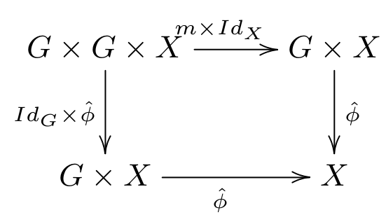
(Here, is the multiplication in , and this is the familiar associativity-type axiom for a group action: acting by a product of two elements in is the same as acting by each one successively.

So the starting point for the paper with Roger Picken was to categorify this. It’s useful, before doing that, to stop and think for a moment about what makes this possible.

First, as stated, this assumed that either is a set, or has an underlying set by way of some faithful forgetful functor: that is, every morphism in corresponds to a unique set map from the elements of to itself. We needed this to describe the groupoid , whose objects are exactly the elements of . The diagram above suggests a different way to think about this. The action diagram lives in the category : we are thinking of as a set together with some structure maps. and the morphism must be in the same category, , for this characterization to make sense.

So in fact, what matters is that the category lived in was closed: that is, it is enriched in itself, so that for any objects , there is an object , the internal hom. In this case, it’s which appears in the diagram. Such an internal hom is supposed to be a dual to ‘s monoidal product (which happens to be the Cartesian product ): this is exactly what lets us talk about .

So really, this construction of a transformation groupoid will work for any closed monoidal category , producing a groupoid in . It may be easier to understand in cases like , the category of topological spaces, where there is indeed a faithful underlying set functor. But although talking explicitly about elements of was useful for intuitively seeing how relates global and local symmetries, it played no particular role in the construction.

Categorify Everything

In the circles I run in, a popular hobby is to “categorify everything“: there are different versions, but what we mean here is to turn ideas expressed in the world of sets into ideas in the world of categories. (Technical aside: all the categories here are assumed to be small). In principle, this is harder than just reproducing all of the above in any old closed monoidal category: the “world” of categories is , which is a closed monoidal 2-category, which is a more complicated notion. This means that doing all the above “strictly” is a special case: all the equalities (like the commutativity of the action square) might in principle be replaced by (natural) isomorphisms, and a good categorification involves picking these to have good properties.

(In our paper, we left this to an appendix, because the strict special case is already interesting, and in any case there are “strictification” results, such as the fact that weak 2-groups are all equivalent to strict 2-groups, which mean that the weak case isn’t as much more general as it looks. For higher -categories, this will fail – which is why we include the appendix to suggest how the pattern might continue).

Why is this interesting to us? Bumping up the “categorical level” appeals for different reasons, but the ones matter most to me have to do with taking low-dimensional (or -codimensional) structures, and finding analogous ones at higher (co)dimension. In our case, the starting point had to do with looking at the symmetries of “higher gauge theories” – which can be used to describe the transport of higher-dimensional surfaces in a background geometry, the way gauge theories can describe the transport of point particles. But I won’t ask you to understand that example right now, as long as you can accept that “what are the global/local symmetries of a category like?” is a possibly interesting question.

So let’s categorify the discussion about symmetry above… To begin with, we can just take our (closed monoidal) category to be , and follow the same construction above. So our first ingredient is a 2-group . As with groups, we can think of a 2-group either as a 2-category with just one object , or as a 1-category with some structure – a group object in , which we’ll call if it comes from a given 2-group. (In our paper, we keep these distinct by using the term “categorical group” for the second. The group axioms amount to saying that we have a monoidal category . Its objects are the morphisms of the 2-group, and the composition becomes the monoidal product .)

(In fact, we often use a third equivalent definition, that of crossed modules of groups, but to avoid getting into that machinery here, I’ll be changing our notation a little.)

2-Group Actions

So, again, there are two ways to talk about an action of a 2-group on some category . One is to define an action as a 2-functor . The object being acted on, , is the unique object – so that the 2-functor amounts to a monoidal functor from the categorical group into . Notice that here we’re taking advantage of the fact that is closed, so that the hom-“sets” are actually categories, and the automorphisms of – invertible functors from to itself – form the objects of a monoidal category, and in fact a categorical group. What’s new, though, is that there are also 2-morphisms – natural transformations between these functors.

To begin with, then, we show that there is a map , which corresponds to the 2-functor , and satisfies an action axiom like the square above, with playing the role of group multiplication. (Again, remember that we’re only talking about the version where this square commutes strictly here – in an appendix of the paper, we talk about the weak version of all this.) This is an intuitive generalization of the situation for groups, but it is slightly more complicated.

The action directly gives three maps. First, functors for each 2-group morphism – each of which consists of a function between objects of , together with a function between morphisms of . Second, natural transformations for 2-morphisms in the 2-group – each of which consists of a function from objects to morphisms of .

On the other hand, is just a functor: it gives two maps, one taking pairs of objects to objects, the other doing the same for morphisms. Clearly, the map is just given by . The map taking pairs of morphisms to morphisms of is less intuitively obvious. Since I already claimed and are equivalent, it should be no surprise that we ought to be able to reconstruct the other two parts of from it as special cases. These are morphism-maps for the functors, (which give or ), and the natural transformation maps (which give or ). In fact, there are only two sensible ways to combine these four bits of information, and the fact that is natural means precisely that they’re the same, so:

Given the above, though, it’s not so hard to see that a 2-group action really involves two group actions: of the objects of on the objects of , and of the morphisms of on objects of . They fit together nicely because objects can be identified with their identity morphisms: furthermore, being a functor gives an action of -objects on -morphisms which fits in between them nicely.

But what of the transformation groupoid? What is the analog of the transformation groupoid, if we repeat its construction in ?

The Transformation Double Category of a 2-Group Action

The answer is that a category (such as a groupoid) internal to is a double category. The compact way to describe it is as a “category in “, with a category of objects and a category of morphisms, each of which of course has objects and morphisms of its own. For the transformation double category, following the same construction as for sets, the object-category is just , and the morphism-category is , and the target functor is just the action map . (The other structure maps that make this into a category in can similarly be worked out by following your nose).

This is fine, but the internal description tends to obscure an underlying symmetry in the idea of double categories, in which morphisms in the object-category and objects in the morphism-category can switch roles, and get a different description of “the same” double category, denoted the “transpose”.

A different approach considers these as two different types of morphism, “horizontal” and “vertical”: they are the morphisms of horizontal and vertical categories, built on the same set of objects (the objects of the object-category). The morphisms of the morphism-category are then called “squares”. This makes a convenient way to draw diagrams in the double category. Here’s a version of a diagram from our paper with the notation I’ve used here, showing what a square corresponding to a morphism looks like:

The square (with the boxed label) has the dashed arrows at the top and bottom for its source and target horizontal morphisms (its images under the source and target functors: the argument above about naturality means they’re well-defined). The vertical arrows connecting them are the source and target vertical morphisms (its images under the source and target maps in the morphism-category).

Horizontal and Vertical Slices of

So by construction, the horizontal category of these squares is just the object-category .  For the same reason, the squares and vertical morphisms, make up the category .

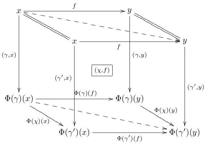
On the other hand, the vertical category has the same objects as , but different morphisms: it’s not hard to see that the vertical category is just the transformation groupoid for the action of the group of -objects on the set of -objects, . Meanwhile, the horizontal morphisms and squares make up the transformation groupoid . These are the object-category and morphism-category of the transpose of the double-category we started with.

We can take this further: if squares aren’t hip enough for you – or if you’re someone who’s happy with 2-categories but finds double categories unfamiliar – the horizontal and vertical categories can be extended to make horizontal and vertical bicategories. They have the same objects and morphisms, but we add new 2-cells which correspond to squares where the boundaries have identity morphisms in the direction we’re not interested in. These two turn out to feel quite different in style.

First, the horizontal bicategory extends by adding 2-morphisms to it, corresponding to morphisms of : roughly, it makes the morphisms of into the objects of a new transformation groupoid, based on the action of the group of automorphisms of the identity in (which ensures the square has identity edges on the sides.) This last point is the only constraint, and it’s not a very strong one since and essentially determine the entire 2-group: the constraint only relates to the structure of .

The constraint for the vertical bicategory is different in flavour because it depends more on the action . Here we are extending a transformation groupoid, . But, for some actions, many morphisms in might just not show up at all. For 1-morphisms , the only 2-morphisms which can appear are those taking to some which has the same effect on as . So, for example, this will look very different if is free (so only automorphisms show up), or a trivial action (so that all morphisms appear).

In the paper, we look at these in the special case of an adjoint action of a 2-group, so you can look there if you’d like a more concrete example of this difference.

Speculative Remarks

The starting point for this was a project (which I talked about a year ago) to do with higher gauge theory – see the last part of the linked post for more detail. The point is that, in gauge theory, one deals with connections on bundles, and morphisms between them called gauge transformations. If one builds a groupoid out of these in a natural way, it turns out to result from the action of a big symmetry group of all gauge transformations on the moduli space of connections.

In higher gauge theory, one deals with connections on gerbes (or higher gerbes – a bundle is essentially a “0-gerbe”). There are now also (2-)morphisms between gauge transformations (and, in higher cases, this continues further), which Roger Picken and I have been calling “gauge modifications”. If we try to repeat the situation for gauge theory, we can construct a 2-groupoid out of these, which expresses this local symmetry. The thing which is different for gerbes (and will continue to get even more different if we move to -gerbes and the corresponding -groupoids) is that this is not the same type of object as a transformation double category.

Now, in our next paper (which this one was written to make possible) we show that the 2-groupoid is actually very intimately related to the transformation double category: that is, the local picture of symmetry for a higher gauge theory is, just as in the lower-dimensional situation, intimately related to a global symmetry of an entire moduli 2-space, i.e. a category. The reason this wasn’t obvious at first is that the moduli space which includes only connections is just the space of objects of this category: the point is that there are really two special kinds of gauge transformations. One should be thought of as the morphisms in the moduli 2-space, and the other as part of the symmetries of that 2-space. The intuition that comes from ordinary gauge theory overlooks this, because the phenomenon doesn’t occur there.

Physically-motivated theories are starting to use these higher-categorical concepts more and more, and symmetry is a crucial idea in physics. What I’ve sketched here is presumably only the start of a pattern in which “symmetry” extends to higher-categorical entities. When we get to 3-groups, our simplifying assumptions that use “strictification” results won’t even be available any more, so we would expect still further new phenomena to show up – but it seems plausible that the tight relation between global and local symmetry will still exist, but in a way that is more subtle, and refines the standard understanding we have of symmetry today.