Theoretical Atlas

One talk at the workshop was nominally a school talk by Laurent Freidel, but it’s interesting and distinctive enough in its own right that I wanted to consider it by itself.  It was based on this paper on the “Principle of Relative Locality”. This isn’t so much a new theory, as an exposition of what ought to happen when one looks at a particular limit of any putative theory that has both quantum field theory and gravity as (different) limits of it. This leads through some ideas, such as curved momentum space, which have been kicking around for a while. The end result is a way of accounting for apparently non-local interactions of particles, by saying that while the particles themselves “see” the interactions as local, distant observers might not.

Whereas Einstein’s gravity describes a regime where Newton’s gravitational constant is important but Planck’s constant is negligible, and (special-relativistic) quantum field theory assumes significant but not.  Both of these assume there is a special velocity scale, given by the speed of light , whereas classical mechanics assumes that all three can be neglected (i.e. and are zero, and is infinite).   The guiding assumption is that these are all approximations to some more fundamental theory, called “quantum gravity” just because it accepts that both and (as well as ) are significant in calculating physical effects.  So GR and QFT incorporate two of the three constants each, and classical mechanics incorporates neither.  The “principle of relative locality” arises when we consider a slightly different approximation to this underlying theory.

This approximation works with a regime where and are each negligible, but the ratio is not – this being related to the Planck mass .  The point is that this is an approximation with no special length scale (“Planck length”), but instead a special energy scale (“Planck mass”) which has to be preserved.   Since energy and momentum are different parts of a single 4-vector, this is also a momentum scale; we expect to see some kind of deformation of momentum space, at least for momenta that are bigger than this scale.  The existence of this scale turns out to mean that momenta don’t add linearly – at least, not unless they’re very small compared to the Planck scale.

So what is “Relative Locality”?  In the paper linked above, it’s stated like so:

Physics takes place in phase space and there is no invariant global projection that gives a description of processes in spacetime.  From their measurements local observers can construct descriptions of particles moving and interacting in a spacetime, but different observers construct different spacetimes, which are observer-dependent slices of phase space.

Motivation

This arises from taking the basic insight of general relativity – the requirement that physical principles should be invariant under coordinate transformations (i.e. diffeomorphisms) – and extend it so that instead of applying just to spacetime, it applies to the whole of phase space.  Phase space (which, in this limit where , replaces the Hilbert space of a truly quantum theory) is the space of position-momentum configurations (of things small enough to treat as point-like, in a given fixed approximation).  Having no means we don’t need to worry about any dynamical curvature of “spacetime” (which doesn’t exist), and having no Planck length means we can blithely treat phase space as a manifold with coordinates valued in the real line (which has no special scale).  Yet, having a special mass/momentum scale says we should see some purely combined “quantum gravity” effects show up.

The physical idea is that phase space is an accurate description of what we can see and measure locally.  Observers (whom we assume small enough to be considered point-like) can measure their own proper time (they “have a clock”) and can detect momenta (by letting things collide with them and measuring the energy transferred locally and its direction).  That is, we “see colors and angles” (i.e. photon energies and differences of direction).  Beyond this, one shouldn’t impose any particular theory of what momenta do: we can observe the momenta of separate objects and see what results when they interact and deduce rules from that.  As an extension of standard physics, this model is pretty conservative.  Now, conventionally, phase space would be the cotangent bundle of spacetime .  This model is based on the assumption that objects can be at any point, and wherever they are, their space of possible momenta is a vector space.  Being a bundle, with a global projection onto (taking to ), is exactly what this principle says doesn’t necessarily obtain.  We still assume that phase space will be some symplectic manifold.   But we don’t assume a priori that momentum coordinates give a projection whose fibres happen to be vector spaces, as in a cotangent bundle.

Now, a symplectic manifold  still looks locally like a cotangent bundle (Darboux’s theorem). So even if there is no universal “spacetime”, each observer can still locally construct a version of “spacetime”  by slicing up phase space into position and momentum coordinates.  One can, by brute force, extend the spacetime coordinates quite far, to distant points in phase space.  This is roughly analogous to how, in special relativity, each observer can put their own coordinates on spacetime and arrive at different notions of simultaneity.  In general relativity, there are issues with trying to extend this concept globally, but it can be done under some conditions, giving the idea of “space-like slices” of spacetime.  In the same way, we can construct “spacetime-like slices” of phase space.

Geometrizing Algebra

Now, if phase space is a cotangent bundle, momenta can be added (the fibres of the bundle are vector spaces).  Some more recent ideas about “quasi-Hamiltonian spaces” (initially introduced by Alekseev, Malkin and Meinrenken) conceive of momenta as “group-valued” – rather than taking values in the dual of some Lie algebra (the way, classically, momenta are dual to velocities, which live in the Lie algebra of infinitesimal translations).  For small momenta, these are hard to distinguish, so even group-valued momenta might look linear, but the premise is that we ought to discover this by experiment, not assumption.  We certainly can detect “zero momentum” and for physical reasons can say that given two things with two momenta , there’s a way of combining them into a combined momentum .  Think of doing this physically – transfer all momentum from one particle to another, as seen by a given observer.  Since the same momentum at the observer’s position can be either coming in or going out, this operation has a “negative” with .

We do have a space of momenta at any given observer’s location – the total of all momenta that can be observed there, and this space now has some algebraic structure.  But we have no reason to assume up front that is either commutative or associative (let alone that it makes momentum space at a given observer’s location into a vector space).  One can interpret this algebraic structure as giving some geometry.  The commutator for gives a metric on momentum space.  This is a bilinear form which is implicitly defined by the “norm” that assigns a kinetic energy to a particle with a given momentum. The associator given by , infinitesimally near where this makes sense, gives a connection.  This defines a “parallel transport” of a finite momentum in the direction of a momentum by saying infinitesimally what happens when adding to .

Various additional physical assumptions – like the momentum-space “duals” of the equivalence principle (that the combination of momenta works the same way for all kinds of matter regardless of charge), or the strong equivalence principle (that inertial mass and rest mass energy per the relation are the same) and so forth can narrow down the geometry of this metric and connection.  Typically we’ll find that it needs to be Lorentzian.  With strong enough symmetry assumptions, it must be flat, so that momentum space is a vector space after all – but even with fairly strong assumptions, as with general relativity, there’s still room for this “empty space” to have some intrinsic curvature, in the form of a momentum-space “dual cosmological constant”, which can be positive (so momentum space is closed like a sphere), zero (the vector space case we usually assume) or negative (so momentum space is hyperbolic).

This geometrization of what had been algebraic is somewhat analogous to what happened with velocities (i.e. vectors in spacetime)) when the theory of special relativity came along.  Insisting that the “invariant” scale be the same in every reference system meant that the addition of velocities ceased to be linear.  At least, it did if you assume that adding velocities has an interpretation along the lines of: “first, from rest, add velocity v to your motion; then, from that reference frame, add velocity w”.  While adding spacetime vectors still worked the same way, one had to rephrase this rule if we think of adding velocities as observed within a given reference frame – this became (scaling so and assuming the velocities are in the same direction).  When velocities are small relative to , this looks roughly like linear addition.  Geometrizing the algebra of momentum space is thought of a little differently, but similar things can be said: we think operationally in terms of combining momenta by some process.  First transfer (group-valued) momentum to a particle, then momentum – the connection on momentum space tells us how to translate these momenta into the “reference frame” of a new observer with momentum shifted relative to the starting point.  Here again, the special momentum scale (which is also a mass scale since a momentum has a corresponding kinetic energy) is a “deformation” parameter – for momenta that are small compared to this scale, things seem to work linearly as usual.

There’s some discussion in the paper which relates this to DSR (either “doubly” or “deformed” special relativity), which is another postulated limit of quantum gravity, a variation of SR with both a special velocity and a special mass/momentum scale, to consider “what SR looks like near the Planck scale”, which treats spacetime as a noncommutative space, and generalizes the Lorentz group to a Hopf algebra which is a deformation of it.  In DSR, the noncommutativity of “position space” is directly related to curvature of momentum space.  In the “relative locality” view, we accept a classical phase space, but not a classical spacetime within it.

Physical Implications

We should understand this scale as telling us where “quantum gravity effects” should start to become visible in particle interactions.  This is a fairly large scale for subatomic particles.  The Planck mass as usually given is about 21 micrograms: small for normal purposes, about the size of a small sand grain, but very large for subatomic particles.  Converting to momentum units with , this is about 6 kg m/s: on the order of the momentum of a kicked soccer ball or so.  For a subatomic particle this is a lot.

This scale does raise a question for many people who first hear this argument, though – that quantum gravity effects should become apparent around the Planck mass/momentum scale, since macro-objects like the aforementioned soccer ball still seem to have linearly-additive momenta.  Laurent explained the problem with this intuition.  For interactions of big, extended, but composite objects like soccer balls, one has to calculate not just one interaction, but all the various interactions of their parts, so the “effective” mass scale where the deformation would be seen becomes where is the number of particles in the soccer ball.  Roughly, the point is that a soccer ball is not a large “thing” for these purposes, but a large conglomeration of small “things”, whose interactions are “fundamental”.  The “effective” mass scale tells us how we would have to alter the physical constants to be able to treat it as a “thing”.  (This is somewhat related to the question of “effective actions” and renormalization, though these are a bit more complicated.)

There are a number of possible experiments suggested in the paper, which Laurent mentioned in the talk.  One involves a kind of “twin paradox” taking place in momentum space.  In “spacetime”, a spaceship travelling a large loop at high velocity will arrive where it started having experienced less time than an observer who remained there (because of the Lorentzian metric) – and a dual phenomenon in momentum space says that particles travelling through loops (also in momentum space) should arrive displaced in space because of the relativity of localization.  This could be observed in particle accelerators where particles make several transits of a loop, since the effect is cumulative.  Another effect could be seen in astronomical observations: if an observer is observing some distant object via photons of different wavelengths (hence momenta), she might “localize” the object differently – that is, the two photons travel at “the same speed” the whole way, but arrive at different times because the observer will interpret the object as being at two different distances for the two photons.

This last one is rather weird, and I had to ask how one would distinguish this effect from a variable speed of light (predicted by certain other ideas about quantum gravity).  How to distinguish such effects seems to be not quite worked out yet, but at least this is an indication that there are new, experimentally detectible, effects predicted by this “relative locality” principle.  As Laurent emphasized, once we’ve noticed that not accepting this principle means making an a priori assumption about the geometry of momentum space (even if only in some particular approximation, or limit, of a true theory of quantum gravity), we’re pretty much obliged to stop making that assumption and do the experiments.  Finding our assumptions were right would simply be revealing which momentum space geometry actually obtains in the approximation we’re studying.

A final note about the physical interpretation: this “relative locality” principle can be discovered by looking (in the relevant limit) at a Lagrangian for free particles, with interactions described in terms of momenta.  It so happens that one can describe this without referencing a “real” spacetime: the part of the action that allows particles to interact when “close” only needs coordinate functions, which can certainly exist here, but are an observer-dependent construct.  The conservation of (non-linear) momenta is specified via a Lagrange multiplier.  The whole Lagrangian formalism for the mechanics of colliding particles works without reference to spacetime.  Now, even though all the interactions (specified by the conservation of momentum terms) happen “at one location”, in that there will be an observer who sees them happening in the momentum space of her own location.  But an observer at a different point may disagree about whether the interaction was local – i.e. happened at a single point in spacetime.  Thus “relativity of localization”.

Again, this is no more bizarre (mathematically) than the fact that distant, relatively moving, observers in special relativity might disagree about simultaneity, whether two events happened at the same time.  They have their own coordinates on spacetime, and transferring between them mixes space coordinates and time coordinates, so they’ll disagree whether the time-coordinate values of two events are the same.  Similarly, in this phase-space picture, two different observers each have a coordinate system for splitting phase space into “spacetime” and “energy-momentum” coordinates, but switching between them may mix these two pieces.  Thus, the two observers will disagree about whether the spacetime-coordinate values for the different interacting particles are the same.  And so, one observer says the interaction is “local in spacetime”, and the other says it’s not.  The point is that it’s local for the particles themselves (thinking of them as observers).  All that’s going on here is the not-very-astonishing fact that in the conventional picture, we have no problem with interactions being nonlocal in momentum space (particles with very different momenta can interact as long as they collide with each other)… combined with the inability to globally and invariantly distinguish position and momentum coordinates.

What this means, philosophically, can be debated, but it does offer some plausibility to the claim that space and time are auxiliary, conceptual additions to what we actually experience, which just account for the relations between bits of matter.  These concepts can be dispensed with even where we have a classical-looking phase space rather than Hilbert space (where, presumably, this is even more true).

…

Edit: On a totally unrelated note, I just noticed this post by Alex Hoffnung over at the n-Category Cafe which gives a lot of detail on issues relating to spans in bicategories that I had begun to think more about recently in relation to developing a higher-gauge-theoretic version of the construction I described for ETQFT. In particular, I’d been thinking about how the 2-group analog of restriction and induction for representations realizes the various kinds of duality properties, where we have adjunctions, biadjunctions, and so forth, in which units and counits of the various adjunctions have further duality. This observation seems to be due to Jim Dolan, as far as I can see from a brief note in HDA II. In that case, it’s really talking about the star-structure of the span (tri)category, but looking at the discussion Alex gives suggests to me that this theme shows up throughout this subject. I’ll have to take a closer look at the draft paper he linked to and see if there’s more to say…

As usual, this write-up process has been taking a while since life does intrude into blogging for some reason.  In this case, because for a little less than a week, my wife and I have been on our honeymoon, which was delayed by our moving to Lisbon.  We went to the Azores, or rather to São Miguel, the largest of the nine islands.  We had a good time, roughly like so:

Now that we’re back, I’ll attempt to wrap up with the summaries of things discussed at the workshop on Higher Gauge Theory, TQFT, and Quantum Gravity.  In the previous post I described talks which I roughly gathered under TQFT and Higher Gauge Theory, but the latter really ramifies out in a few different ways.  As began to be clear before, higher bundles are classified by higher cohomology of manifolds, and so are gerbes – so in fact these are two slightly different ways of talking about the same thing.  I also remarked, in the summary of Konrad Waldorf’s talk, the idea that the theory of gerbes on a manifold is equivalent to ordinary gauge theory on its loop space – which is one way to make explicit the idea that categorification “raises dimension”, in this case from parallel transport of points to that of 1-dimensional loops.  Next we’ll expand on that theme, and then finally reach the “Quantum Gravity” part, and draw the connection between this and higher gauge theory toward the end.

Gerbes and Cohomology

The very first workshop speaker, in fact, was Paolo Aschieri, who has done a lot of work relating noncommutative geometry and gravity.  In this case, though, he was talking about noncommutative gerbes, and specifically referred to this work with some of the other speakers.  To be clear, this isn’t about gerbes with noncommutative group , but about gerbes on noncommutative spaces.  To begin with, it’s useful to express gerbes in the usual sense in the right language.  In particular, he explain what a gerbe on a manifold is in concrete terms, giving Hitchin’s definition (viz).  A gerbe can be described as “a cohomology class” but it’s more concrete to present it as:

• a collection of line bundles associated with double overlaps 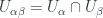.  Note this gets an algebraic structure (multiplication of bundles is pointwise , with an inverse given by the dual, , so we can require…
• , which helps define…
• transition functions on triple overlaps , which are sections of 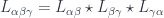.  If this product is trivial, there’d be a 1-cocycle condition here, but we only insist on the 2-cocycle condition…
• 

This is a -gerbe on a commutative space.  The point is that one can make a similar definition for a noncommutative space.  If the space is associated with the algebra of smooth functions, then a line bundle is a module for , so if is noncommutative (thought of as a “space” ), a “bundle over is just defined to be an -module.  One also has to define an appropriate “covariant derivative” operator on this module, and the -product must be defined as well, and will be noncommutative (we can think of it as a deformation of the above).  The transition functions are sections: that is, elements of the modules in question.  his means we can describe a gerbe in terms of a big stack of modules, with a chosen algebraic structure, together with some elements.  The idea then is that gerbes can give an interpretation of cohomology of noncommutative spaces as well as commutative ones.

Mauro Spera spoke about a point of view of gerbes based on “transgressions”.  The essential point is that an -gerbe on a space can be seen as the obstruction to patching together a family of  -gerbes.  Thus, for instance, a 0-gerbe is a -bundle, which is to say a complex line bundle.  As described above, a 1-gerbe can be understood as describing the obstacle to patching together a bunch of line bundles, and the obstacle is the ability to find a cocycle satisfying the requisite conditions.  This obstacle is measured by the cohomology of the space.  Saying we want to patch together -gerbes on the fibre.  He went on to discuss how this manifests in terms of obstructions to string structures on manifolds (already discussed at some length in the post on Hisham Sati’s school talk, so I won’t duplicate here).

A talk by Igor Bakovic, “Stacks, Gerbes and Etale Groupoids”, gave a way of looking at gerbes via stacks (see this for instance).  The organizing principle is the classification of bundles by the space maps into a classifying space – or, to get the category of principal -bundles on, the category , where is the category of sheaves on and is the classifying topos of -sets.  (So we have geometric morphisms between the toposes as the objects.)  Now, to get further into this, we use that is equivalent to the category of Étale spaces over – this is a refinement of the equivalence between bundles and presheaves.  Taking stalks of a presheaf gives a bundle, and taking sections of a bundle gives a presheaf – and these operations are adjoint.

The issue at hand is how to categorify this framework to talk about 2-bundles, and the answer is there’s a 2-adjunction between the 2-category of such things, and , the 2-category of fibred categories over .  (That is, instead of looking at “sheaves of sets”, we look at “sheaves of categories” here.)  The adjunction, again, involves talking stalks one way, and taking sections the other way.  One hard part of this is getting a nice definition of “stalk” for stacks (i.e. for the “sheaves of categories”), and a good part of the talk focused on explaining how to get a nice tractable definition which is (fibre-wise) equivalent to the more natural one.

Bakovic did a bunch of this work with Branislav Jurco, who was also there, and spoke about “Nonabelian Bundle 2-Gerbes“.  The paper behind that link has more details, which I’ve yet to entirely absorb, but the essential point appears to be to extend the description of “bundle gerbes” associated to crossed modules up to 2-crossed modules.  Bundles, with a structure-group , are classified by the cohomology with coefficients in ; and whereas “bundle-gerbes” with a structure-crossed-module can likewise be described by cohomology .  Notice this is a bit different from the description in terms of higher cohomology for a -gerbe, which can be understood as a bundle-gerbe using the shifted crossed module (when is abelian.  The goal here is to generalize this part to nonabelian groups, and also pass up to “bundle 2-gerbes” based on a 2-crossed module, or crossed complex of length 2, as I described previously for Joao Martins’ talk.  This would be classified in terms of cohomology valued in the 2-crossed module.  The point is that one can describe such a thing as a bundle over a fibre product, which (I think – I’m not so clear on this part) deals with the same structure of overlaps as the higher cohomology in the other way of describing things.

Finally,  a talk that’s a little harder to classify than most, but which I’ve put here with things somewhat related to string theory, was Alexander Kahle‘s on “T-Duality and Differential K-Theory”, based on work with Alessandro Valentino.  This uses the idea of the differential refinement of cohomology theories – in this case, K-theory, which is a generalized cohomology theory, which is to say that K-theory satisfies the Eilenberg-Steenrod axioms (with the dimension axiom relaxed, hence “generalized”).  Cohomology theories, including generalized ones, can have differential refinements, which pass from giving topological to geometrical information about a space.  So, while K-theory assigns to a space the Grothendieck ring of the category of vector bundles over it, the differential refinement of K-theory does the same with the category of vector bundles with connection.  This captures both local and global structures, which turns out to be necessary to describe fields in string theory – specifically, Ramond-Ramond fields.  The point of this talk was to describe what happens to these fields under T-duality.  This is a kind of duality in string theory between a theory with large strings and small strings.  The talk describes how this works, where we have a manifold with fibres at each point with fibres strings of radius and with radius .  There’s a correspondence space 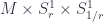, which has projection maps down into the two situations.  Fields, being forms on such a fibration, can be “transferred” through this correspondence space by a “pull-back and push-forward” (with, in the middle, a wedge with a form that mixes the two directions, ).  But to be physically the right kind of field, these “forms” actually need to be representing cohomology classes in the differential refinement of K-theory.

Quantum Gravity etc.

Now, part of the point of this workshop was to try to build, or anyway maintain, some bridges between the kind of work in geometry and topology which I’ve been describing and the world of physics.  There are some particular versions of physical theories where these ideas have come up.  I’ve already touched on string theory along the way (there weren’t many talks about it from a physicist’s point of view), so this will mostly be about a different sort of approach.

Benjamin Bahr gave a talk outlining this approach for our mathematician-heavy audience, with his talk on “Spin Foam Operators” (see also for instance this paper).  The point is that one approach to quantum gravity has a theory whose “kinematics” (the description of the state of a system at a given time) is described by “spin networks” (based on gauge theory), as described back in the pre-school post.  These span a Hilbert space, so the “dynamical” issue of such models is how to get operators between Hilbert spaces from “foams” that interpolate between such networks – that is, what kind of extra data they might need, and how to assign amplitudes to faces and edges etc. to define an operator, which (assuming a “local” theory where distant parts of the foam affect the result independently) will be of the form:

where is a particular complex (foam), is a way of assigning irreps to faces of the foam, and is the assignment of intertwiners to edges.  Later on, one can take a discrete version of a path integral by summing over all these .  Here we have a product over faces and one over vertices, with an amplitude assigned (somehow – this is the issue) to faces.  The trace is over all the representation spaces assigned to the edges that are incident to a vertex (this is essentially the only consistent way to assign an amplitude to a vertex).  If we also consider spacetimes with boundary, we need some amplitudes at the boundary edges, as well.  A big part of the work with such models is finding such amplitudes that meet some nice conditions.

Some of these conditions are inherently necessary – to ensure the theory is invariant under gauge transformations, or (formally) changing orientations of faces.  Others are considered optional, though to me “functoriality” (that the way of deriving operators respects the gluing-together of foams) seems unavoidable – it imposes that the boundary amplitudes have to be found from the in one specific way.  Some other nice conditions might be: that depends only on the topology of (which demands that the operators be projections); that is invariant under subdivision of the foam (which implies the amplitudes have to be ).

Assuming all these means the only choice is exactly which sub-projection is of the projection onto the gauge-invariant part of the representation space for the faces attached to edge .  The rest of the talk discussed this, including some examples (models for BF-theory, the Barrett-Crane model and the more recent EPRL/FK model), and finished up by discussing issues about getting a nice continuum limit by way of “coarse graining”.

On a related subject, Bianca Dittrich spoke about “Dynamics and Diffeomorphism Symmetry in Discrete Quantum Gravity”, which explained the nature of some of the hard problems with this sort of discrete model of quantum gravity.  She began by asking what sort of models (i.e. which choices of amplitudes) in such discrete models would actually produce a nice continuum theory – since gravity, classically, is described in terms of spacetimes which are continua, and the quantum theory must look like this in some approximation.  The point is to think of these as “coarse-graining” of a very fine (perfect, in the limit) approximation to the continuum by a triangulation with a very short length-scale for the edges.  Coarse graining means discarding some of the edges to get a coarser approximation (perhaps repeatedly).  If the happens to be triangulation-independent, then coarse graining makes no difference to the result, nor does the converse process of refining the triangulation.  So one question is:  if we expect the continuum limit to be diffeomorphism invariant (as is General Relativity), what does this say at the discrete level?  The relation between diffeomorphism invariance and triangulation invariance has been described by Hendryk Pfeiffer, and in the reverse direction by Dittrich et al.

Actually constructing the dynamics for a system like this in a nice way (“canonical dynamics with anomaly-free constraints”) is still a big problem, which Bianca suggested might be approached by this coarse-graining idea.  Now, if a theory is topological (here we get the link to TQFT), such as electromagnetism in 2D, or (linearized) gravity in 3D, coarse graining doesn’t change much.  But otherwise, changing the length scale means changing the action for the continuum limit of the theory.  This is related to renormalization: one starts with a “naive” guess at a theory, then refines it (in this case, by the coarse-graining process), which changes the action for the theory, until arriving at (or approximating to) a fixed point.  Bianca showed an example, which produces a really huge, horrible action full of very complicated terms, which seems rather dissatisfying.  What’s more, she pointed out that, unless the theory is topological, this always produces an action which is non-local – unlike the “naive” discrete theory.  That is, the action can’t be described in terms of a bunch of non-interacting contributions from the field at individual points – instead, it’s some function which couples the field values at distant points (albeit in a way that falls off exponentially as the points get further apart).

In a more specific talk, Aleksandr Mikovic discussed “Finiteness and Semiclassical Limit of EPRL-FK Spin Foam Models”, looking at a particular example of such models which is the (relatively) new-and-improved candidate for quantum gravity mentioned above.  This was a somewhat technical talk, which I didn’t entirely follow, but  roughly, the way he went at this was through the techniques of perturbative QFT.  That is, by looking at the theory in terms of an “effective action”, instead of some path integral over histories with action – which looks like .  Starting with some classical history – a stationary point of the action – the effective action is an integral over small fluctuations around it of .

He commented more on the distinction between the question of triangulation independence (which is crucial for using spin foams to give invariants of manifolds) and the question of whether the theory gives a good quantum theory of gravity – that’s the “semiclassical limit” part.  (In light of the above, this seems to amount to asking if “diffeomorphism invariance” really extends through to the full theory, or is only approximately true, in the limiting case).  Then the “finiteness” part has to do with the question of getting decent asymptotic behaviour for some of those weights mentioned above so as to give a nice effective action (if not necessarily triangulation independence).  So, for instance, in the Ponzano-Regge model (which gives a nice invariant for manifolds), the vertex amplitudes are found by the 6j-symbols of representations.  The asymptotics of the 6j symbols then becomes an issue – Alekandr noted that to get a theory with a nice effective action, those 6j-symbols need to be scaled by a certain factor.  This breaks triangulation independence (hence means we don’t have a good manifold invariant), but gives a physically nicer theory.  In the case of 3D gravity, this is not what we want, but as he said, there isn’t a good a-priori reason to think it can’t give a good theory of 4D gravity.

Now, making a connection between these sorts of models and higher gauge theory, Aristide Baratin spoke about “2-Group Representations for State Sum Models”.  This is a project Baez, Freidel, and Wise, building on work by Crane and Sheppard (see my previous post, where Derek described the geometry of the representation theory for some 2-groups).  The idea is to construct state-sum models where, at the kinematical level, edges are labelled by 2-group representations, faces by intertwiners, and tetrahedra by 2-intertwiners.  (This assumes the foam is a triangulation – there’s a certain amount of back-and-forth in this area between this, and the Poincaré dual picture where we have 4-valent vertices).  He discussed this in a couple of related cases – the Euclidean and Poincaré 2-groups, which are described by crossed modules with base groups or respectively, acting on the abelian group (of automorphisms of the identity) in the obvious way.  Then the analogy of the 6j symbols above, which are assigned to tetrahedra (or dually, vertices in a foam interpolating two kinematical states), are now 10j symbols assigned to 4-simplexes (or dually, vertices in the foam).

One nice thing about this setup is that there’s a good geometric interpretation of the kinematics – irreducible representations of these 2-groups pick out orbits of the action of the relevant on .  These are “mass shells” – radii of spheres in the Euclidean case, or proper length/time values that pick out hyperboloids in the Lorentzian case of .  Assigning these to edges has an obvious geometric meaning (as a proper length of the edge), which thus has a continuous spectrum.  The areas and volumes interpreting the intertwiners and 2-intertwiners start to exhibit more of the discreteness you see in the usual formulation with representations of the groups themselves.  Finally, Aristide pointed out that this model originally arose not from an attempt to make a quantum gravity model, but from looking at Feynman diagrams in flat space (a sort of “quantum flat space” model), which is suggestively interesting, if not really conclusively proving anything.

Finally, Laurent Freidel gave a talk, “Classical Geometry of Spin Network States” which was a way of challenging the idea that these states are exclusively about “quantum geometries”, and tried to give an account of how to interpret them as discrete, but classical.  That is, the quantization of the classical phase space (the cotangent bundle of connections-mod-gauge) involves first a discretization to a spin-network phase space , and then a quantization to get a Hilbert space , and the hard part is the first step.  The point is to see what the classical phase space is, and he describes it as a (symplectic) quotient , which starts by assigning $T^*(SU(2))$ to each edge, then reduced by gauge transformations.  The puzzle is to interpret the states as geometries with some discrete aspect.

The answer is that one thinks of edges as describing (dual) faces, and vertices as describing some polytopes.  For each , there’s a -dimensional “shape space” of convex polytopes with -faces and a given fixed area .  This has a canonical symplectic structure, where lengths and interior angles at an edge are the canonically conjugate variables.  Then the whole phase space describes ways of building geometries by gluing these things (associated to vertices) together at the corresponding faces whenever the two vertices are joined by an edge.  Notice this is a bit strange, since there’s no particular reason the faces being glued will have the same shape: just the same area.  An area-1 pentagon and an area-1 square associated to the same edge could be glued just fine.  Then the classical geometry for one of these configurations is build of a bunch of flat polyhedra (i.e. with a flat metric and connection on them).  Measuring distance across a face in this geometry is a little strange.  Given two points inside adjacent cells, you measure orthogonal distance to the matched faces, and add in the distance between the points you arrive at (orthogonally) – assuming you glued the faces at the centre.  This is a rather ugly-seeming geometry, but it’s symplectically isomorphic to the phase space of spin network states – so it’s these classical geometries that spin-foam QG is a quantization of.  Maybe the ugliness should count against this model of quantum gravity – or maybe my aesthetic sense just needs work.

(Laurent also gave another talk, which was originally scheduled as one of the school talks, but ended up being a very interesting exposition of the principle of “Relativity of Localization”, which is hard to shoehorn into the themes I’ve used here, and was anyway interesting enough that I’ll devote a separate post to it.)

Now for a more sketchy bunch of summaries of some talks presented at the HGTQGR workshop.  I’ll organize this into a few themes which appeared repeatedly and which roughly line up with the topics in the title: in this post, variations on TQFT, plus 2-group and higher forms of gauge theory; in the next post, gerbes and cohomology, plus talks on discrete models of quantum gravity and suchlike physics.

TQFT and Variations

I start here for no better reason than the personal one that it lets me put my talk first, so I’m on familiar ground to start with, for which reason also I’ll probably give more details here than later on.  So: a TQFT is a linear representation of the category of cobordisms – that is, a (symmetric monoidal) functor , in the notation I mentioned in the first school post.  An Extended TQFT is a higher functor , representing a category of cobordisms with corners into a higher category of k-Vector spaces (for some definition of same).  The essential point of my talk is that there’s a universal construction that can be used to build one of these at , which relies on some way of representing into , whose objects are groupoids, and whose morphisms in are pairs of groupoid homomorphisms .  The 2-morphisms have an analogous structure.  The point is that there’s a 2-functor which is takes representations of groupoids, at the level of objects; for morphisms, there is a “pull-push” operation that just uses the restricted and induced representation functors to move a representation across a span; the non-trivial (but still universal) bit is the 2-morphism map, which uses the fact that the restriction and induction functors are bi-ajdoint, so there are units and counits to use.  A construction using gauge theory gives groupoids of connections and gauge transformations for each manifold or cobordism.  This recovers a form of the Dijkgraaf-Witten model.  In principle, though, any way of getting a groupoid (really, a stack) associated to a space functorially will give an ETQFT this way.  I finished up by suggesting what would need to be done to extend this up to higher codimension.  To go to codimension 3, one would assign an object (codimension-3 manifold) a 3-vector space which is a representation 2-category of 2-groupoids of connections valued in 2-groups, and so on.  There are some theorems about representations of n-groupoids which would need to be proved to make this work.

The fact that different constructions can give groupoids for spaces was used by the next speaker, Thomas Nicklaus, whose talk described another construction that uses the I mentioned above.  This one produces “Equivariant Dijkgraaf-Witten Theory”.  The point is that one gets groupoids for spaces in a new way.  Before, we had, for a space a groupoid whose objects are -connections (or, put another way, bundles-with-connection) and whose morphisms are gauge transformations.  Now we suppose that there’s some group which acts weakly (i.e. an action defined up to isomorphism) on .  We think of this as describing “twisted bundles” over .  This is described by a quotient stack (which, as a groupoid, gets some extra isomorphisms showing where two objects are related by the -action).  So this gives a new map , and applying gives a TQFT.  The generating objects for the resulting 2-vector space are “twisted sectors” of the equivariant DW model.  There was some more to the talk, including a description of how the DW model can be further mutated using a cocycle in the group cohomology of , but I’ll let you look at the slides for that.

Next up was Jamie Vicary, who was talking about “(1,2,3)-TQFT”, which is another term for what I called “Extended” TQFT above, but specifying that the objects are 1-manifolds, the morphisms 2-manifolds, and the 2-morphisms are 3-manifolds.  He was talking about a theorem that identifies oriented TQFT’s of this sort with “anomaly-free modular tensor categories” – which is widely believed, but in fact harder than commonly thought.  It’s easy enough that such a TQFT corresponds to a MTC – it’s the category assigned to the circle.  What’s harder is showing that the TQFT’s are equivalent functors iff the categories are equivalent.  This boils down, historically, to the difficulty of showing the category is rigid.  Jamie was talking about a project with Bruce Bartlett and Chris Schommer-Pries, whose presentation of the cobordism category (described in the school post) was the basis of their proof.

Part of it amounts to giving a description of the TQFT in terms of certain string diagrams.  Jamie kindly credited me with describing this point of view to him: that the codimension-2 manifolds in a TQFT can be thought of as “boundaries in space” – codimension-1 manifolds are either time-evolving boundaries, or else slices of space in which the boundaries live; top-dimension cobordisms are then time-evolving slices of space-with-boundary.  (This should be only a heuristic way of thinking – certainly a generic TQFT has no literal notion of “time-evolution”, though in that (2+1) quantum gravity can be seen as a TQFT, there’s at least one case where this picture could be taken literally.)  Then part of their proof involves showing that the cobordisms can be characterized by taking vector spaces on the source and target manifolds spanned by the generating objects, and finding the functors assigned to cobordisms in terms of sums over all “string diagrams” (particle worldlines, if you like) bounded by the evolving boundaries.  Jamie described this as a “topological path integral”.  Then one has to describe the string diagram calculus – ridigidy follows from the “yanking” rule, for instance, and this follows from Morse theory as in Chris’ presentation of the cobordism category.

There was a little more discussion about what the various properties (proved in a similar way) imply.  One is “cloaking” – the fact that a 2-morphism which “creates a handle” is invisible to the string diagrams in the sense that it introduces a sum over all diagrams with a string “looped” around the new handle, but this sum gives a result that’s equal to the original map (in any “pivotal” tensor category, as here).

Chronologically before all these, one of the first talks on such a topic was by Rafael Diaz, on Homological Quantum Field Theory, or HLQFT for short, which is a rather different sort of construction.  Remember that Homotopy QFT, as described in my summary of Tim Porter’s school sessions, is about linear representations of what I’ll for now call , whose morphisms are -dimensional cobordisms equipped with maps into a space up to homotopy.  HLQFT instead considers cobordisms equipped with maps taken up to homology.

Specifically, there’s some space , say a manifold, with some distinguished submanifolds (possibly boundary components; possibly just embedded submanifolds; possibly even all of for a degenerate case).  Then we define to have objects which are -manifolds equipped with maps into which land on the distinguished submanifolds (to make composition work nicely, we in fact assume they map to a single point).  Morphisms in are trickier, and look like : a cobordism in this category is likewise equipped with a map from its boundary into which recovers the maps on its objects.  That is a homology class of maps from to , which agrees with .  This forms a monoidal category as with standard cobordisms.  Then HLQFT is about representations of this category.  One simple case Rafael described is the dimension-1 case, where objects are (ordered sets of) points equipped with maps that pick out chosen submanifolds of , and morphisms are just braids equipped with homology classes of “paths” joining up the source and target submanifolds.  Then a representation might, e.g., describe how to evolve a homology class on the starting manifold to one on the target by transporting along such a path-up-to-homology.  In higher dimensions, the evolution is naturally more complicated.

A slightly looser fit to this section is the talk by Thomas Krajewski, “Quasi-Quantum Groups from Strings” (see this) – he was talking about how certain algebraic structures arise from “string worldsheets”, which are another way to describe cobordisms.  This does somewhat resemble the way an algebraic structure (Frobenius algebra) is related to a 2D TQFT, but here the string worldsheets are interacting with 3-form field, (the curvature of that 2-form field of string theory) and things needn’t be topological, so the result is somewhat different.

Part of the point is that quantizing such a thing gives a higher version of what happens for quantizing a moving particle in a gauge field.  In the particle case, one comes up with a line bundle (of which sections form the Hilbert space) and in the string case one comes up with a gerbe; for the particle, this involves associated 2-cocycle, and for the string a 3-cocycle; for the particle, one ends up producing a twisted group algebra, and for the string, this is where one gets a “quasi-quantum group”.  The algebraic structures, as in the TQFT situation, come from, for instance, the “pants” cobordism which gives a multiplication and a comultiplication (by giving maps or the reverse, where is the object assigned to a circle).

There is some machinery along the way which I won’t describe in detail, except that it involves a tricomplex of forms – the gradings being form degree, the degree of a cocycle for group cohomology, and the number of overlaps.  As observed before, gerbes and their higher versions have transition functions on higher numbers of overlapping local neighborhoods than mere bundles.  (See the paper above for more)

Higher Gauge Theory

The talks I’ll summarize here touch on various aspects of higher-categorical connections or 2-groups (though at least one I’ll put off until later).  The division between this and the section on gerbes is a little arbitrary, since of course they’re deeply connected, but I’m making some judgements about emphasis or P.O.V. here.

Apart from giving lectures in the school sessions, John Huerta also spoke on “Higher Supergroups for String Theory”, which brings “super” (i.e. -graded) objects into higher gauge theory.  There are “super” versions of vector spaces and manifolds, which decompose into “even” and “odd” graded parts (a.k.a. “bosonic” and “fermionic” parts).  Thus there are “super” variants of Lie algebras and Lie groups, which are like the usual versions, except commutation properties have to take signs into account (e.g. a Lie superalgebra’s bracket is commutative if the product of the grades of two vectors is odd, anticommutative if it’s even).  Then there are Lie 2-algebras and 2-groups as well – categories internal to this setting.  The initial question has to do with whether one can integrate some Lie 2-algebra structures to Lie 2-group structures on a spacetime, which depends on the existence of some globally smooth cocycles.  The point is that when spacetime is of certain special dimensions, this can work, namely dimensions 3, 4, 6, and 10.  These are all 2 more than the real dimensions of the four real division algebras, , , and .  It’s in these dimensions that Lie 2-superalgebras can be integrated to Lie 2-supergroups.  The essential reason is that a certain cocycle condition will hold because of the properties of a form on the Clifford algebras that are associated to the division algebras.  (John has some related material here and here, though not about the 2-group case.)

Since we’re talking about higher versions of Lie groups/algebras, an important bunch of concepts to categorify are those in representation theory.  Derek Wise spoke on “2-Group Representations and Geometry”, based on work with Baez, Baratin and Freidel, most fully developed here, but summarized here.  The point is to describe the representation theory of Lie 2-groups, in particular geometrically.  They’re to be represented on (in general, infinite-dimensional) 2-vector spaces of some sort, which is chosen to be a category of measurable fields of Hilbert spaces on some measure space, which is called (intended to resemble, but not exactly be the same as, , the space of “functors into from the space , the way Kapranov-Voevodsky 2-vector spaces can be described as ).  The first work on this was by Crane and Sheppeard, and also Yetter.  One point is that for 2-groups, we have not only representations and intertwiners between them, but 2-intertwiners between these.  One can describe these geometrically – part of which is a choice of that measure space .

This done, we can say that a representation of a 2-group is a 2-functor , where is seen as a one-object 2-category.  Thinking about this geometrically, if we concretely describe by the crossed module , defines an action of on , and a map into the character group, which thereby becomes a -equivariant bundle.  One consequence of this description is that it becomes possible to distinguish not only irreducible representations (bundles over a single orbit) and indecomposible ones (where the fibres are particularly simple homogeneous spaces), but an intermediate notion called “irretractible” (though it’s not clear how much this provides).  An intertwining operator between reps over and can be described in terms of a bundle of Hilbert spaces – which is itself defined over the pullback of and seen as -bundles over .  A 2-intertwiner is a fibre-wise map between two such things.  This geometric picture specializes in various ways for particular examples of 2-groups.  A physically interesting one, which Crane and Sheppeard, and expanded on in that paper of [BBFW] up above, deals with the Poincaré 2-group, and where irreducible representations live over mass-shells in Minkowski space (or rather, the dual of ).

Moving on from 2-group stuff, there were a few talks related to 3-groups and 3-groupoids.  There are some new complexities that enter here, because while (weak) 2-categories are all (bi)equivalent to strict 2-categories (where things like associativity and the interchange law for composing 2-cells hold exactly), this isn’t true for 3-categories.  The best strictification result is that any 3-category is (tri)equivalent to a Gray category – where all those properties hold exactly, except for the interchange law for horizontal and vertical compositions of 2-cells, which is replaced by an “interchanger” isomorphism with some coherence properties.  John Barrett gave an introduction to this idea and spoke about “Diagrams for Gray Categories”, describing how to represent morphisms, 2-morphisms, and 3-morphisms in terms of higher versions of “string” diagrams involving (piecewise linear) surfaces satisfying some properties.  He also carefully explained how to reduce the dimensions in order to make them both clearer and easier to draw.  Bjorn Gohla spoke on “Mapping Spaces for Gray Categories”, but since it was essentially a shorter version of a talk I’ve already posted about, I’ll leave that for now, except to point out that it linked to the talk by Joao Faria Martins, “3D Holonomy” (though see also this paper with Roger Picken).

The point in Joao’s talk starts with the fact that we can describe holonomies for 3-connections on 3-bundles valued in Gray-groups (i.e. the maximally strict form of a general 3-group) in terms of Gray-functors 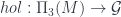.  Here, is the fundamental 3-groupoid of , which turns points, paths, homotopies of paths, and homotopies of homotopies into a Gray groupoid (modulo some technicalities about “thin” or “laminated”  homotopies) and is a gauge Gray-group.  Just as a 2-group can be represented by a crossed module, a Gray (3-)group can be represented by a “2-crossed module” (yes, the level shift in the terminology is occasionally confusing).  This is a chain of groups , where acts on the other groups, together with some structure maps (for instance, the Peiffer commutator for a crossed module becomes a lifting ) which all fit together nicely.  Then a tri-connection can be given locally by forms valued in the Lie algebras of these groups: in  .  Relating the global description in terms of and local description in terms of is a matter of integrating forms over paths, surfaces, or 3-volumes that give the various -morphisms of .  This sort of construction of parallel transport as functor has been developed in detail by Waldorf and Schreiber (viz. these slides, or the full paper), some time ago, which is why, thematically, they’re the next two speakers I’ll summarize.

Konrad Waldorf spoke about “Abelian Gauge Theories on Loop Spaces and their Regression”.  (For more, see two papers by Konrad on this)  The point here is that there is a relation between two kinds of theories – string theory (with -field) on a manifold , and ordinary gauge theory on its loop space .  The relation between them goes by the name “regression” (passing from gauge theory on to string theory on ), or “transgression”, going the other way.  This amounts to showing an equivalence of categories between [principal -bundles with connection on ] and [-gerbes with connection on ].  This nicely gives a way of seeing how gerbes “categorify” bundles, since passing to the loop space – whose points are maps means a holonomy functor is now looking at objects (points in ) which would be morphisms in the fundamental groupoid of , and morphisms which are paths of loops (surfaces in which trace out homotopies).  So things are shifted by one level.  Anyway, Konrad explained how this works in more detail, and how it should be interpreted as relating connections on loop space to the -field in string theory.

Urs Schreiber kicked the whole categorification program up a notch by talking about -Connections and their Chern-Simons Functionals .  So now we’re getting up into -categories, and particularly -toposes (see Jacob Lurie’s paper, or even book if so inclined to find out what these are), and in particular a “cohesive topos”, where derived geometry can be developed (Urs suggested people look here, where a bunch of background is collected). The point is that -topoi are good for talking about homotopy theory.  We want a setting which allows all that structure, but also allows us to do differential geometry and derived geometry.  So there’s a “cohesive” -topos called , of “sheaves” (in the -topos sense) of -groupoids on smooth manifolds.  This setting is the minimal common generalization of homotopy theory and differential geometry.

This is about a higher analog of this setup: since there’s a smooth classifying space (in fact, a Lie groupoid) for -bundles, , there’s also an equivalence between categories of -principal bundles, and (of functors into ).  Moreover, there’s a similar setup with for bundles with connection.  This can be described topologically, or there’s also a “differential refinement” to talk about the smooth situation.  This equivalence lives within a category of (smooth) sheaves of groupoids.  For higher gauge theory, we want a higher version as in described above.  Then we should get an equivalence – in this cohesive topos – of and a category of –-gerbes.

Then the part about the  “Chern-Simons functionals” refers to the fact that CS theory for a manifold (which is a kind of TQFT) is built using an action functional that is found as an integral of the forms that describe some -connection over the manifold.  (Then one does a path-integral of this functional over all connections to find partition functions etc.)  So the idea is that for these higher -gerbes, whose classifying spaces we’ve just described, there should be corresponding functionals.  This is why, as Urs remarked in wrapping up, this whole picture has an explicit presentation in terms of forms.  Actually, in terms of Cech-cocycles (due to the fact we’re talking about gerbes), whose coefficients are taken in sheaves of complexes (this is the derived geometry part) of differential forms whose coefficients are in -algebroids (the -groupoid version of Lie algebras, since in general we’re talking about a theory with gauge -groupoids now).

Whew!  Okay, that’s enough for this post.  Next time, wrapping up blogging the workshop, finally.

Continuing from the previous post, there are a few more lecture series from the school to talk about.

Higher Gauge Theory

The next was John Huerta’s series on Higher Gauge Theory from the point of view of 2-groups.  John set this in the context of “categorification”, a slightly vague program of replacing set-based mathematical ideas with category-based mathematical ideas.  The general reason for this is to get an extra layer of “maps between things”, or “relations between relations”, etc. which tend to be expressed by natural transformations.  There are various ways to go about this, but one is internalization: given some sort of structure, the relevant example in this case being “groups”, one has a category , and can define a 2-group as a “category internal to “.  So a 2-group has a group of objects, a group of morphisms, and all the usual maps (source and target for morphisms, composition, etc.) which all have to be group homomorphisms.  It should be said that this all produces a “strict 2-group”, since the objects necessarily form a group here.  In particular, satisfies group axioms “on the nose” – which is the only way to satisfy them for a group made of the elements of a set, but for a group made of the elements of a category, one might require only that it commute up to isomorphism.  A weak 2-group might then be described as a “weak model” of the theory of groups in , but this whole approach is much less well-understood than the strict version as one goes to general n-groups.

Now, as mentioned in the previous post, there is a 1-1 correspondence between 2-groups and crossed modules (up to equivalence): given a crossed module , there’s a 2-group whose objects are and whose morphisms are ; given a 2-group with objects , there’s a crossed module .  (The action acts on a morphism in such as way as to act by multiplication on its source and target).  Then, for instance, the Peiffer identity for crossed modules (see previous post) is a consequence of the fact that composition of morphisms is supposed to be a group homomorphism.

Looking at internal categories in [your favourite setting here] isn’t the only way to do categorification, but it does produce some interesting examples.  Baez-Crans 2-vector spaces are defined this way (in ), and built using these are Lie 2-algebras.  Looking for a way to integrate Lie 2-algebras up to Lie 2-groups (which are internal categories in Lie groups) brings us back to the current main point.  This is the use of 2-groups to do higher gauge theory.  This requires the use of “2-bundles”.  To explain these, we can say first of all that a “2-space” is an internal category in (whether that be manifolds, or topological spaces, or what-have-you), and that a (locally trivial) 2-bundle should have a total 2-space , a base 2-space , and a (functorial) projection map , such that there’s some open cover of by neighborhoods where locally the bundle “looks like” , where is the fibre of the bundle.  In the bundle setting, “looks like” means “is isomorphic to” by means of isomorphisms .  With 2-bundles, it’s interpreted as “is equivalent to” in the categorical sense, likewise by maps .

Actually making this precise is a lot of work when is a general 2-space – even defining open covers and setting up all the machinery properly is quite hard.  This has been done, by Toby Bartels in his thesis, but to keep things simple, John restricted his talk to the case where is just an ordinary manifold (thought of as a 2-space which has only identity morphisms).   Then a key point is that there’s an analog to how (principal) -bundles (where as a -set) are classified up to isomorphism by the first Cech cohomology of the manifold, .  This works because one can define transition functions on double overlaps , by .  Then these will automatically satisfy the 1-cocycle condidion ( on the triple overlap ) which means they represent a cohomology class .

A comparable thing can be said for the “transition functors” for a 2-bundle – they’re defined superficially just as above, except that being functors, we can now say there’s a natural isomorphism , and it’s these , defined on triple overlaps, which satisfy a 2-cocycle condition on 4-fold intersections (essentially, the two ways to compose them to collapse into agree).  That is, we have and which fit together nicely.  In particular, we have an element of the second Cech cohomology of : “principal -bundles are classified by second Cech cohomology of “.  This sort of thing ties in to an ongoing theme of the later talks, the relationship between gerbes and higher cohomology – a 2-bundle corresponds to a “gerbe”, or rather a “1-gerbe”.  (The consistent terminology would have called a bundle a “0-gerbe”, but as usual, terminology got settled before the general pattern was understood).

Finally, having defined bundles, one usually defines connections, and so we do the same with 2-bundles.  A connection on a bundle gives a parallel transport operation for paths in , telling how to identify the fibres at points along by means of a functor , thinking of as a category with one object, and where is the path groupoid whose objects are points in and whose morphisms are paths (up to “thin” homotopy). At least, it does so once we trivialize the bundle around , anyway, to think of it as locally – in general we need to get the transition functions involved when we pass into some other local neighborhood.  A connection on a 2-bundle is similar, but tells how to parallel transport fibres not only along paths, but along homotopies of paths, by means of , where is seen as a 2-category with one object, and now has 2-morphisms which are (essentially) homotopies of paths.

Just as connections can be described by 1-forms valued in , which give by integrating, a similar story exists for 2-connections: now we need a 1-form valued in and a 2-form valued in .  These need to satisfy some relations, essentially that the curvature of has to be controlled by .   Moreover, that is related to the -field of string theory, as I mentioned in the post on the pre-school… But really, this is telling us about the Lie 2-algebra associated to , and how to integrate it up to the group!

Infinite Dimensional Lie Theory and Higher Gauge Theory

This series of talks by Christoph Wockel returns us to the question of “integrating up” to a Lie group from a Lie algebra , which is seen as the tangent space of at the identity.  This is a well-understood, well-behaved phenomenon when the Lie algebras happen to be finite dimensional.  Indeed the classification theorem for the classical Lie groups can be got at in just this way: a combinatorial way to characterize Lie algebras using Dynkin diagrams (which describe the structure of some weight lattice), followed by a correspondence between Lie algebras and Lie groups.  But when the Lie algebras are infinite dimensional, this just doesn’t have to work.  It may be impossible to integrate a Lie algebra up to a full Lie group: instead, one can only get a little neighborhood of the identity.  The point of such infinite-dimensional groups, and ultimately their representation theory, is to deal with string groups that have to do with motions of extended objects.  Christoph Wockel was describing a result which says that, going to 2-groups, this problem can be overcome.  (See the relevant paper here.)

The first lecture in the series presented some background on a setting for infinite dimensional manifolds.  There are various approaches, a popular one being Frechet manifolds, but in this context, the somewhat weaker notion of locally convex spaces is sufficient.  These are “locally modelled” by (infinite dimensional) locally convex vector spaces, the way finite dimensonal manifolds are locally modelled by Euclidean space.  Being locally convex is enough to allow them to support a lot of differential calculus: one can find straight-line paths, locally, to define a notion of directional derivative in the direction of a general vector.  Using this, one can build up definitions of differentiable and smooth functions, derivatives, and integrals, just by looking at the restrictions to all such directions.  Then there’s a fundamental theorem of calculus, a chain rule, and so on.

At this point, one has plenty of differential calculus, and it becomes interesting to bring in Lie theory.  A Lie group is defined as a group object in the category of manifolds and smooth maps, just as in the finite-dimensional case.  Some infinite-dimensional Lie groups of interest would include: , the group of diffeomorphisms of some compact manifold ; and the group of smooth functions from into some (finite-dimensional) Lie group (perhaps just ), with the usual pointwise multiplication.  These are certainly groups, and one handy fact about such groups is that, if they have a manifold structure near the identity, on some subset that generates as a group in a nice way, you can extend the manifold structure to the whole group.  And indeed, that happens in these examples.

Well, next we’d like to know if we can, given an infinite dimensional Lie algebra , “integrate up” to a Lie group – that is, find a Lie group for which is the “infinitesimal” version of .  One way this arises is from central extensions.  A central extension of Lie group by is an exact sequence where (the image of) is in the centre of .  The point here is that extends .  This setup makes is a principal -bundle over .

Now, finding central extensions of Lie algebras is comparatively easy, and given a central extension of Lie groups, one always falls out of the induced maps.  There will be an exact sequence of Lie algebras, and now the special condition is that there must exist a continuous section of the second map.  The question is to go the other way: given one of these, get back to an extension of Lie groups.  The problem of finding extensions of by , in particular as a problem of finding a bundle with connection having specified curvature, which brings us back to gauge theory.  One type of extension is the universal cover of , which appears as , so that the fibre is .

In general, whether an extension can exist comes down to a question about a cocycle: that is, if there’s a function which is locally smooth (i.e. in some neighborhood in ), and is a cocyle (so that ), by the same sorts of arguments we’ve already seen a bit of.  For this reason, central extensions are classified by the cohomology group .  The cocycle enables a “twisting” of the multiplication associated to a nontrivial loop in , and is used to construct (by specifying how multiplication on lifts to ).  Given a  2-cocycle at the Lie algebra level (easier to do), one would like to lift that up the Lie group.  It turns out this is possible if the period homomorphism – which takes a chain (with ) to the integral of the original cocycle on it, – lands in a discrete subgroup of . A popular example of this is when is just , and the discrete subgroup is (or, similarly, and respectively).  This business of requiring a cocycle to be integral in this way is sometimes called a “prequantization” problem.

So suppose we wanted to make the “2-connected cover”  as a central extension: since will be abelian, this is conceivable.  If the dimension of is finite, this is trivial (since in finite dimensions), which is why we need some theory  of infinite-dimensional manifolds.  Moreover, though, this may not work in the context of groups: the in the extension above needs to be a “twisting” of associativity, not multiplication, being lifted from .  Such twistings come from the THIRD cohomology of (see here, e.g.), and describe the structure of 2-groups (or crossed modules, whichever you like).  In fact, the solution (go read the paper for more if you like) to define a notion of central extension for 2-groups (essentially the same as the usual definition, but with maps of 2-groups, or crossed modules, everywhere).  Since a group is a trivial kind of 2-group (with only trivial automorphisms of any element), the usual notion of central extension turns out to be a special case.  Then by thinking of and as crossed modules, one can find a central extension which is like the 2-connected cover we wanted – though it doesn’t work as an extension of groups because we think of as the base group of the crossed module, and as the second group in the tower.

The pattern of moving to higher group-like structures, higher cohomology, and obstructions to various constructions ran all through the workshop, and carried on in the next school session…

Higher Spin Structures in String Theory

Hisham Sati gave just one school-lecture in addition to his workshop talk, but it was packed with a lot of material.  This is essentially about cohomology and the structures on manifolds to which cohomology groups describe the obstructions.  The background part of the lecture referenced this book by Fridrich, and the newer parts were describing some of Sati’s own work, in particular a couple of papers with Schreiber and Stasheff (also see this one).

The basic point here is that, for physical reasons, we’re often interested in putting some sort of structure on a manifold, which is really best described in terms of a bundle.  For instance, a connection or spin connection on spacetime lets us transport vectors or spinors, respectively, along paths, which in turn lets us define derivatives.  These two structures really belong on vector bundles or spinor bundles.  Now, if these bundles are trivial, then one can make the connections on them trivial as well by gauge transformation.  So having nontrivial bundles really makes this all more interesting.  However, this isn’t always possible, and so one wants to the obstruction to being able to do it.  This is typically a class in one of the cohomology groups of the manifold – a characteristic class.  There are various examples: Chern classes, Pontrjagin classes, Steifel-Whitney classes, and so on, each of which comes in various degrees .  Each one corresponds to a different coefficient group for the cohomology groups – in these examples, the groups and which are the limits of the unitary and orthogonal groups (such as )

The point is that these classes are obstructions to building certain structures on the manifold – which amounts to finding sections of a bundle.  So for instance, the first Steifel-Whitney classes, of a bundle are related to orientations, coming from cohomology with coefficients in .  Orientations for the manifold can be described in terms of its tangent bundle, which is an -bundle (tangent spaces carry an action of the rotation group).  Consider , where we have actually .  The group has two elements, and there are two types of line bundle on the circle : ones with a nowhere-zero section, like the trivial bundle; and ones without, like the Moebius strip.  The circle is orientable, because its tangent bundle is of the first sort.

Generally, an orientation can be put on if the tangent bundle, as a map , can be lifted to a map – that is, it’s “secretly” an -bundle – the special orthogonal group respects orientation, which is what the determinant measures.  Its two values, , are what’s behind the two classes of bundles.  (In short, this story relates to the exact sequence ; in just the same way we have big groups , , and so forth.)

So spin structures have a story much like the above, but where the exact sequence plays a role – the spin groups are the universal covers (which are all double-sheeted covers) of the special rotation groups.  A spin structure on some bundle , let’s say represented by  is thus, again, a lifting to .  The obstruction to doing this (the thing which must be zero for the lifting to exist) is the second Stiefel-Whitney class, .  Hisham Sati also explained the example of “generalized” spin structures in these terms.  But the main theme is an analogous, but much more general, story for other cohomology groups as obstructions to liftings of some sort of structures on manifolds.  These may be bundles, for the lower-degree cohomology, or they may be gerbes or n-bundles, for higher-degree, but the setup is roughly the same.

The title’s term “higher spin structures” comes from the fact that we’ve so far had a tower of classifying spaces (or groups), , and so on.  Then the problem of putting various sorts of structures on has been turned into the problem of lifting a map up this tower.  At each point, the obstruction to lifting is some cohomology class with coefficients in the groups (, , etc.)  So when are these structures interesting?

This turns out to bring up another theme, which is that of special dimensions – it’s just not true that the same phenomena happen in every dimension.  In this case, this has to do with the homotopy groups  – of and its cousins.  So it turns out that the homotopy group (which is the same as as long as is bigger than ) follows a pattern, where if , and if .  The fact that this pattern repeats mod-8 is one form of the (real) Bott Periodicity theorem.  These homotopy groups reflect that, wherever there’s nontrivial homotopy in some dimension, there’s an obstruction to contracting maps into from such a sphere.

All of this plays into the question of what kinds of nontrivial structures can be put on orthogonal bundles on manifolds of various dimensions.  In the dimensions where these homotopy groups are non-trivial, there’s an obstruction to the lifting, and therefore some interesting structure one can put on which may or may not exist.  Hisham Sati spoke of “killing” various homotopy groups – meaning, as far as I can tell, imposing conditions which get past these obstructions.  In string theory, his application of interest, one talks of “anomaly cancellation” – an anomaly being the obstruction to making these structures.  The first part of the punchline is that, since these are related to nontrivial cohomology groups, we can think of them in terms of defining structures on n-bundles or gerbes.  These structures are, essentially, connections – they tell us how to parallel-transport objects of various dimensions.  It turns out that the homotopy group is related to parallel transport along -dimensional surfaces in , which can be thought of as the world-sheets of -dimensional “particles” (or rather, “branes”).

So, for instance, the fact that is nontrivial means there’s an obstruction to a lifting in the form of a class in , which has to do with spin structure – as above.  “Cancelling” this “anomaly” means that for a theory involving such a spin structure to be well-defined, then this characteristic class for must be zero.  The fact that is nontrivial means there’s an obstruction to a lifting in the form of a class in .  This has to do with “string bundles”, where the string group is a higher analog of in exactly the sense we’ve just described.  If such a lifting exists, then there’s a “string-structure” on which is compatible with the spin structure we lifted (and with the orientation a level below that).  Similarly, being nontrivial, by way of an obstruction in , means there’s an interesting notion of “five-brane” structure, and a group, and so on.  Personally, I think of these as giving a geometric interpretation for what the higher cohomology groups actually mean.

A slight refinement of the above, and actually more directly related to “cancellation” of the anomalies, is that these structures can be defined in a “twisted” way: given a cocycle in the appropriate cohomology group, we can ask that a lifting exist, not on the nose, but as a diagram commuting only up to a higher cell, which is exactly given by the cocycle.  I mentioned, in the previous section, a situation where the cocycle gives an associator, so that instead of being exactly associative, a structure has a “twisted” associativity.  This is similar, except we’re twisting the condition that makes a spin structure (or higher spin structure) well-defined.  So if has the wrong characteristic class, we can only define one of these twisted structures at that level.

This theme of higher cohomology and gerbes, and their geometric interpretation, was another one that turned up throughout the talks in the workshop…

And speaking of that: coming up soon, some descriptions of the actual workshop.

I’d like to continue describing the talks that made up the HGTQGR workshop, in particular the ones that took place during the school portion of the event.  I’ll save one “school” session, by Laurent Freidel, to discuss with the talks because it seems to more nearly belong there. This leaves five people who gave between two and four lectures each over a period of a few days, all intermingled. Here’s a very rough summary in the order of first appearance:

2D Extended TQFT

Chris Schommer-Pries gave the longest series of talks, about the classification of 2D extended TQFT’s.  A TQFT is a kind of topological invariant for manifolds, which has a sort of “locality” property, in that you can decompose the manifold, compute the invariant on the parts, and find the whole by gluing the pieces back together.  This is expressed by saying it’s a monoidal functor , where the “locality” property is now functoriality property that composition is preserved.  The key thing here is the cobordism category , which has objects (d-1)-dimensional manifolds, and morphisms d-dimensional cobordisms (manifolds with boundary, where the objects are components of the boundary).  Then a closed d-manifold is just a cobordism from $latex\emptyset$ to itself.

Making this into a category is actually a bit nontrivial: gluing bits of smooth manifolds, for instance, won’t necessarily give something smooth.  There are various ways of handling this, such as giving the boundaries “collars”, but Chris’ preferred method is to give boundaries (and, ultimately, corners, etc.) a”halation”.  This word originally means the halo of light around bright things you sometimes see in photos, but in this context, a halation for is an equivalence class of embeddings into neighborhoods .  The equivalence class says two such embeddings into and are equivalent if there’s a compatible refinement into some common that embeds into both and .  The idea is that a halation is a kind of d-dimensional “halo”, or the “germ of a d-manifold” around .  Then gluing compatibly along (d-1)-boundaries with halations ensures that we get smooth d-manifolds.  (One can also extend this setup so that everything in sight is oriented, or has some other such structure on it.)

In any case, an extended TQFT will then mean an n-functor , where is some symmetric monoidal n-category (which is supposed to be similar to ).  Its exact nature is less important than that of , which has:

• 0-Morphisms (i.e. Objects): 0-manifolds (collections of points)
• 1-Morphisms: 1-dimensional cobordisms between 0-manifolds (curves)
• 2-Morphisms: 2-dim cobordisms with corners between 1-Morphisms (surfaces with boundary)
• …
• d-Morphisms: d-dimensional cobordisms between (d-1)-Morphisms (n-manifolds with corners), up to isomorphism

(Note: the distinction between “Bord” and “Cobord” is basically a matter of when a given terminology came in.  “Cobordism” and “Bordism”, unfortunately, mean the same thing, except that “bordism” has become popular more recently, since the “co” makes it sound like it’s the opposite category of something else.  This is kind of regrettable, but that’s what happened.  Sorry.)

The crucial point, is that Chris wanted to classify all such things, and his approach to this is to give a presentation of .  This is based on stuff in his thesis.  The basic idea is to use Morse theory, and its higher-dimensional generalization, Cerf theory.  The idea is that one can put a Morse function  on a cobordism (essentially, a well-behaved “time order” on points) and look at its critical points.  Classifying these tells us what the generators for the category of cobordisms must be: there need to be enough to capture all the most general sorts of critical points.

Cerf theory does something similar, but one dimension up: now we’re talking about “stratified” families of Morse functions.  Again one studies critical points, but, for instance, on a 2-dim surface, there can be 1- and 0-dimensional parts of the set of cricical points.  In general, this gets into the theory of higher-dimensional singularities, catastrophe theory, and so on.  Each extra dimension one adds means looking at how the sets of critical points in the previous dimension can change over “time” (i.e. within some stratified family of Cerf functions).  Where these changes themselves go through critical points, one needs new generators for the various j-morphisms of the cobordism category.  (See some examples of such “catastrophes”, such as folds, cusps, swallowtails, etc. linked from here, say.)  Showing what such singularities can be like in the “generic” situation, and indeed, even defining “generic” in a way that makes sense in any dimension, required some discussion of jet bundles.  These are generalizations of tangent bundles that capture higher derivatives the way tangent bundles capture first-derivatives.  The essential point is that one can find a way to decompose these into a direct sum of parts of various dimensions (capturing where various higher derivatives are zero, say), and these will eventually tell us the dimension of a set of critical points for a Cerf function.

Now, this gives a characterization of what cobordisms can be like – part of the work in the theorem is to show that this is sufficient: that is, given a diagram showing the critical points for some Morse/Cerf function, one needs to be able to find the appropriate generators and piece together the cobordism (possibly a closed manifold) that it came from.  Chris showed how this works – a slightly finicky process involving cutting a diagram of the singular points (with some extra labelling information) into parts, and using a graphical calculus to work out how pasting works – and showed an example reconstruction of a surface this way.  This amounts to a construction of an equivalence between an “abstract” cobordism category given in terms of generators (and relations) which come from Cerf theory, and the concrete one.  The theorem then says that there’s a correspondence between equivalence classes of 2D cobordisms, and certain planar diagrams, up to some local moves.  To show this properly required a digression through some theory of symmetric monoidal bicategories, and what the right notion of equivalence for them is.

This all done, the point is that has a characterization in terms of a universal property, and so any ETQFT amounts to a certain kind of object in (corresponding to the image of the point – the generating object in ).  For instance, in the oriented situation this object needs to be “fully dualizable”: it should have a dual (the point with opposite orientation), and a whole bunch of maps that specify the duality: a cobordism from to nothing (just the “U”-shaped curve), which has a dual – and some 2-D cobordisms which specify that duality, and so on.  Specifying all this dualizability structure amounts to giving the image of all the generators of cobordisms, and determines the functors , and vice versa.

This is a rapid summary of six hours of lectures, of course, so for more precise versions of these statements, you may want to look into Chris’ thesis as linked above.

Homotopy QFT and the Crossed Menagerie

The next series of lectures in the school was Tim Porter’s, about relations between Homotopy Quantum Field Theory (HQFT) and various sort of crossed gizmos.  HQFT is an idea introduced by Vladimir Turaev, (see his paper with Tim here, for an intro, though Turaev also now has a book on the subject).  It’s intended to deal with similar sorts of structures to TQFT, but with various sorts of extra structure.  This structure is related to the “Crossed Menagerie”, on which Tim has written an almost unbelievably extensive bunch of lecture notes, of which a special short version was made for this lecture series that’s a mere 350 pages long.

Anyway, the cobordism category described above is replaced by one Tim called (see above comment about “bord” and “cobord”, which mean the same thing).  Again, this has d-dimensional cobordisms as its morphisms and (d-1)-dimensional manifolds as its objects, but now everything in sight is equipped with a map into a space – almost.  So an object is , and a morphism is a cobordism with a homotopy class of maps which are compatible with the ones at the boundaries.  Then just as a d-TQFT is a representation (i.e. a functor) of into , a -HQFT is a representation of .

The motivating example here is when , the classifying space of a group.  These spaces are fairly complicated when you describe them as built from gluing cells (in homotopy theory, one typically things of spaces as something like CW-complexes: a bunch of cells in various dimensions glued together with face maps etc.), but has the property that its fundamental group is , and all other homotopy groups are trivial (ensuring this part is what makes the cellular decomposition description tricky).

The upshot is that there’s a correspondence between (homotopy classes of) maps (this makes a good alternative definition of the classifying space, though one needs to ).  Since a map from the fundamental group into amounts to a flat principal -bundle, we can say that is a category of manifolds and cobordisms carrying such a bundle.  This gets us into gauge theory.

But we can go beyond and into higher gauge theory (and other sorts of structures) by picking other sorts of .  To begin with, notice that the correspondence above implies that mapping into means that when we take maps up to homotopy, we can only detect the fundamental group of , and not any higher homotopy groups.  We say we can only detect the “homotopy 1-type” of the space.  The “homotopy n-type” of a given space is just the first homotopy groups .  Alternatively, an “n-type” is an equivalence class of spaces which all have the same such groups.  Or, again, an “n-type” is a particular representative of one of these classes where these are the only nonzero homotopy groups.

The point being that if we’re considering maps up to homotopy, we may only be detecting the n-type of (and therefore may as well assume is an n-type in the last sense when it’s convenient).  More precisely, there are “Postnikov functors” which take a space and return the corresponding n-type.  This can be done by gluing in “patches” of higher dimensions to “fill in the holes” which are measured by the higher homotopy groups (in general, the result is infinite dimensional as a cell complex).  Thus, there are embeddings , which get along with the obvious chain

There was a fairly nifty digression here explaining how this is a “coskeleton” of , in that is a right adjoint to the “n-skeleton” functor (which throws away cells above dimension n, not homotopy groups), so that .  To really explain it properly, though I would have to really explain what that is (it refers to maps in the category of simplicial sets, which are another nice model of spaces up to homotopy).  This digression would carry us away from higher gauge theory, which is where I’m going.

One thing to say is that if is d-dimensional, then any HQFT is determined entirely by the d-type of .  Any extra jazz going on in ‘s higher homotopy groups won’t be detected when we’re only mapping a d-dimensional space into it.  So one might as well assume that is just a d-type.

We want to say we can detect a homotopy n-type of a space if, for example, where is an “n-group”.  A handy way to account for this is in terms of a “crossed complex”.  The first nontrivial example of this would be a crossed module, which consists of

• Two groups, and with
• A map and
• An action of on by automorphisms,
• all such that action looks as much like conjugation as possible:
  • (so that is -equivariant)
  • (the “Peiffer identity”)

This definition looks a little funny, but it does characterize “2-groups” in the sense of categories internal to (the definition used elsewhere), by taking to be the group of objects, and the group of automorphisms of the identity of .  In the description of John Huerta’s lectures, I’ll get back to how that works.

The immediate point is that there are a bunch of natural examples of crossed modules.  For instance: from normal subgroups, where is inclusion and the action really is conjugation; from fibrations, using fundamental groups of base and fibre; from a canonical case where   and takes everything to the identity; from modules, taking to be a -module as an abelian group and again.  The first and last give the classical intuition of these guys: crossed modules are simultaneous generalizations of (a) normal subgroups of , and (b) -modules.

There are various other examples, but the relevant thing here is a theorem of MacLane and Whitehead, that crossed modules model all connected homotopy 2-types.  That is, there’s a correspondence between crossed modules up to isomorphism and 2-types.  Of course, groups model 1-types: any group is the fundmental group for a 1-type, and any 1-type is the classifying space for some group.  Likewise, any crossed module determines a 2-type, and vice versa.  So this theorem suggests why crossed modules might deserve to be called “2-groups” even if they didn’t naturally line up with the alternative definition.

To go up to 3-types and 4-types, the intuitive idea is: “do for crossed modules what we did for groups”.  That is, instead of a map of groups , we consider a map of crossed modules (which is given by a pair of maps between the groups in each) and so forth.  The resulting structure is a square diagram in with a bunch of actions.  Each of these maps is the map for a crossed module.  (We can think of the normal subgroup situation: there are two normal subgroups of , and in each of them, the intersection is normal, so it determines a crossed module).  This is a “crossed square”, and things like this correspond exactly to homotopy 3-types.  This works roughly as before, since there is a notion of a classifying space where , and similarly on for crossed n-cubes.   We can carry on in this way to define a “crossed n-cube”, which correspond to homotopy (n+1)-types.  The correspondence is a little bit more fiddly than it was for groups, but it still exists: any (n+1)-type is the classifying space for a crossed n-cube, and any such crossed n-cube has an (n+1)-type for its classifying space.

This correspondence is the point here.  As we said, when looking at HQFT’s from , we may as well assume that is a d-type.  But then, it’s a classifying space for some crossed (d-1)-cube.  This is a sensible sort of to use in an HQFT, and it ends up giving us a theory which is related to higher gauge theory: a map up to homotopy, where is a crossed n-cube will correspond to the structure of a flat -bundle on , and similarly for cobordisms.  HQFT’s let us look at the structure of this structured cobordism category by means of its linear representations.  Now, it may be that this crossed-cube point of view isn’t the best way to look at , but it is there, and available.

To say more about this, I’ll have to talk more directly about higher gauge theory in its own terms – which I’ll do in part IIb, since this is already pretty long.