Why Higher Geometric Quantization
The largest single presentation was a pair of talks on “The Motivation for Higher Geometric Quantum Field Theory” by Urs Schreiber, running to about two and a half hours, based on these notes. This was probably the clearest introduction I’ve seen so far to the motivation for the program he’s been developing for several years. Broadly, the idea is to develop a higher-categorical analog of geometric quantization (GQ for short).
One guiding idea behind this is that we should really be interested in quantization over (higher) stacks, rather than merely spaces. This leads inexorably to a higher-categorical version of GQ itself. The starting point, though, is that the defining features of stacks capture two crucial principles from physics: the gauge principle, and locality. The gauge principle means that we need to keep track not just of connections, but gauge transformations, which form respectively the objects and morphisms of a groupoid. “Locality” means that these groupoids of configurations of a physical field on spacetime is determined by its local configuration on regions as small as you like (together with information about how to glue together the data on small regions into larger regions).
Some particularly simple cases can be described globally: a scalar field gives the space of all scalar functions, namely maps into 

More generally, physicists think of a field theory as given by a fibre bundle 


More generally, a field theory gives a procedure 


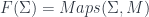

The Yoneda lemma says that, for reasonable notions of “space”, the category 
All of the above is the classical situation: the next issue is how to quantize such a theory. It involves a generalization of Geometric Quantization (GQ for short). Now a physicist who actually uses GQ will find this perspective weird, but it flows from just the same logic as the usual method.
In ordinary GQ, you have some classical system described by a phase space, a manifold 


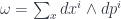
Then one wants to build a Hilbert space describing the quantum analog of the system, but in fact, you need a little more than 

Since the crucial geometric thing here is a bundle over the moduli space, when the space is a stack, and in the context of higher gauge theory, it’s natural to seek analogous constructions using higher bundles. This would involve, instead of a (pre-)symplectic 2-form 

Now, maps between Hilbert spaces in QG come from Lagrangian correspondences – these might be maps of moduli spaces, but in general they consist of a “space of trajectories” equipped with maps into a space of incoming and outgoing configurations. This is a span of pre-symplectic spaces (equipped with pre-quantum line bundles) that satisfies some nice geometric conditions which make it possible to push a section of said line bundle through the correspondence. Since each prequantum line bundle can be seen as maps out of the configuration space into a classifying space (for 
This much is about as far as Urs got in his talk, but the notes go further, talking about how to extend this to infinity-stacks, and how the Dold-Kan correspondence tells us nicer descriptions of what we get when linearizing – since quantization puts us into an Abelian category.
I enjoyed these talks, although they were long and Urs came out looking pretty exhausted, because while I’ve seen several others on this program, this was the first time I’ve seen it discussed from the beginning, with a lot of motivation. This was presumably because we had a physically-minded part of the audience, whereas I’ve mostly seen these for mathematicians, and usually they come in somewhere in the middle and being more time-limited miss out some of the details and the motivation. The end result made it quite a natural development. Overall, very helpful!
